クイックスタートガイド

このノートブックでは,流線トポロジー解析のライブラリである psiclone の使い方を見ていきます.

ライブラリの基本情報と読み込み

このチュートリアルでは,psiclone>=0.4.2 を仮定しています.psiclone のバージョンは,pip show か,もしくは psiclone.version を見ることで調べられます.

2025/04/01 時点での最新版は v0.4.2 になります.

%pip show psiclone
Name: psiclone
Version: 0.4.2
Summary: Toolbox for Topological Flow Data Analysis using COT Representations
Home-page: https://github.com/t-uda/psiclone
Author: Tomoki Uda
Author-email: uda0@sci.u-toyama.ac.jp
License: MIT
Location: /opt/build/repo/.venv/lib/python3.12/site-packages
Requires: matplotlib, msgpack, nbformat, networkx, numpy, plotly, scipy
Required-by: 
Note: you may need to restart the kernel to use updated packages.
import psiclone

help(psiclone.version)
Help on module psiclone.version in psiclone:

NAME
    psiclone.version

FUNCTIONS
    version()

VERSION
    0.4.2

FILE
    /opt/build/repo/.venv/lib/python3.12/site-packages/psiclone/version.py

何か分からないことがあった時は,上の例のように一度 help(...) を試してみると良いでしょう.(これは python に限らない極めて初歩的かつ一般的なアドバイスです.)

help(psiclone)
Help on package psiclone:

NAME
    psiclone - Toolbox for Topological Flow Data Analysis using COT Representations

PACKAGE CONTENTS
    compatibility (package)
    cot
    data (package)
    experimental (package)
    psi2tree
    reeb (package)
    test (package)
    util (package)
    version
    visualization (package)

FILE
    /opt/build/repo/.venv/lib/python3.12/site-packages/psiclone/__init__.py

このように,psiclone がいくつかのサブパッケージからなることが分かります.ここでは,reeb, visualization を予め読み込んでおきます.

import psiclone.reeb
import psiclone.visualization

入力データ形式の取り扱い

データの読み込み

さて,本格的なチュートリアルに入って行きましょう.まず,データの読み書き等の処理にはもちろん numpy が便利です.また,可視化のために matplotlibnetworkx があると便利です.

import matplotlib.pyplot as plt
import networkx
import numpy

入力データ GrayscaleImage

レーブグラフを計算する際の典型的な入力データは \(n \times m\) 実スカラー配列です.これは GrayscaleImage クラスで扱います.せっかくですから,最初だけ help も見ておきましょう.

help(psiclone.data.GrayscaleImage)
Help on class GrayscaleImage in module psiclone.data.image:

class GrayscaleImage(psiclone.data.abstract_graph.AbstractGraph)
 |  GrayscaleImage(array, *, adjacency=array([[0, 1],
 |         [1, 0]], dtype=int32))
 |
 |  A `GrayscaleImage` object represents an `(n, m)`-shaped scalar array.
 |  This object inherits from `AbstractGraph` and is regarded as a lattice graph.
 |
 |  Nodes, edges and link_table are compatible with those of `Geometry` graphs.
 |  Nodes are pixels locating at the 2D integer lattice. Compared to typical
 |  lattice graphs, the adjacency of `GrayscaleImage` is generalized in the sense
 |  that any lattice point is connected to points in its reference ball neighborhood.
 |  The ball neighborhood is specified by `adjacency` parameter and no entities
 |  of the links are maintained. This nontypical adjacency structure is intended
 |  to deal with topological noises in grayscale images, and to avoid overuse of
 |  memory in the case where the datasize and the ball neighborhood are large.
 |
 |  Parameters
 |  ---------
 |  array : `numpy.ndarray`
 |      A two-dimensional numeric array representing a gray-scale image.
 |
 |  adjacency : `numpy.ndarray`, default=`four_points_adjacency()`
 |      A two-dimensional numeric array representing the lattice adjacency.
 |
 |  Notes
 |  -----
 |  The `adjacency` parameter is intended to use one of the following functions generating such an array.
 |
 |  - `box_adjacency(r)`: Connects all lattice points within a box of radius `r`.
 |  - `ball_adjacency(p, r)`: Connects all lattice points within an L^p ball of radius `r`.
 |  - `four_points_adjacency()`: Equivalent to `ball_adjacency(1, 1)` (default).
 |  - `eight_points_adjacency()`: Equivalent to `box_adjacency(1)`
 |
 |  Method resolution order:
 |      GrayscaleImage
 |      psiclone.data.abstract_graph.AbstractGraph
 |      builtins.object
 |
 |  Methods defined here:
 |
 |  __init__(self, array, *, adjacency=array([[0, 1],
 |         [1, 0]], dtype=int32))
 |      Initialize self.  See help(type(self)) for accurate signature.
 |
 |  is_in_bound(self, i, j)
 |
 |  to_geometry(self)
 |      Convert a given 2D array `pict` to a grid geometry.
 |      An edge in a grid geometry links four-point neighbors,
 |      whereas a node in a grid geometry consists of properties
 |      `{'x': i, 'y': j, 'level': pict[i, j], 'geotype': 0}`.
 |
 |      Returns
 |      -------
 |      geometry : `psiclone.data.Geometry`
 |          A grid geometry.
 |
 |  ----------------------------------------------------------------------
 |  Class methods defined here:
 |
 |  create_graph()
 |      Factory method of GrayscaleImage.
 |
 |  ----------------------------------------------------------------------
 |  Readonly properties defined here:
 |
 |  data
 |
 |  edges
 |
 |  link_table
 |
 |  nodes
 |
 |  ----------------------------------------------------------------------
 |  Data and other attributes defined here:
 |
 |  MockLinkTable = <class 'psiclone.data.image.GrayscaleImage.MockLinkTab...
 |      A mock link table of GrayscaleImage without maintaining its Edge entities.
 |
 |
 |  __abstractmethods__ = frozenset()
 |
 |  ----------------------------------------------------------------------
 |  Methods inherited from psiclone.data.abstract_graph.AbstractGraph:
 |
 |  to_network(self)
 |
 |  ----------------------------------------------------------------------
 |  Data descriptors inherited from psiclone.data.abstract_graph.AbstractGraph:
 |
 |  __dict__
 |      dictionary for instance variables
 |
 |  __weakref__
 |      list of weak references to the object

ヘルプに GrayscaleImage(array, *, ......) と書いて行があることに着目してください.これはこのクラスの初期化方法を表しています.これにより,配列を引数として与えて初期化できることが分かります.実際にやってみましょう.

data = numpy.arange(12).reshape((3, 4))
img = psiclone.data.GrayscaleImage(data)

GrayscaleImage オブジェクトは AbstractGraph を継承しており,グラフ構造を持っています.

img.nodes
[Point(id=np.int64(0), level=np.int64(0), x=np.int64(0), y=np.int64(0), geotype=np.int64(1), order=np.float64(-2.498091544796509)),
 Point(id=np.int64(1), level=np.int64(1), x=np.int64(1), y=np.int64(0), geotype=np.int64(1), order=np.float64(-2.1587989303424644)),
 Point(id=np.int64(2), level=np.int64(2), x=np.int64(2), y=np.int64(0), geotype=np.int64(1), order=np.float64(-1.5707963267948966)),
 Point(id=np.int64(3), level=np.int64(3), x=np.int64(3), y=np.int64(0), geotype=np.int64(1), order=np.float64(-0.982793723247329)),
 Point(id=np.int64(4), level=np.int64(4), x=np.int64(0), y=np.int64(1), geotype=np.int64(1), order=np.float64(-2.896613990462929)),
 Point(id=np.int64(5), level=np.int64(5), x=np.int64(1), y=np.int64(1), geotype=np.int64(0), order=np.float64(nan)),
 Point(id=np.int64(6), level=np.int64(6), x=np.int64(2), y=np.int64(1), geotype=np.int64(0), order=np.float64(nan)),
 Point(id=np.int64(7), level=np.int64(7), x=np.int64(3), y=np.int64(1), geotype=np.int64(1), order=np.float64(-0.4636476090008061)),
 Point(id=np.int64(8), level=np.int64(8), x=np.int64(0), y=np.int64(2), geotype=np.int64(1), order=np.float64(2.896613990462929)),
 Point(id=np.int64(9), level=np.int64(9), x=np.int64(1), y=np.int64(2), geotype=np.int64(1), order=np.float64(2.677945044588987)),
 Point(id=np.int64(10), level=np.int64(10), x=np.int64(2), y=np.int64(2), geotype=np.int64(1), order=np.float64(1.5707963267948966)),
 Point(id=np.int64(11), level=np.int64(11), x=np.int64(3), y=np.int64(2), geotype=np.int64(1), order=np.float64(0.4636476090008061))]
list(img.edges)
[<psiclone.data.graph.Edge at 0x7f5816169c40>,
 <psiclone.data.graph.Edge at 0x7f5815f01100>,
 <psiclone.data.graph.Edge at 0x7f5815d6a9f0>,
 <psiclone.data.graph.Edge at 0x7f581607e870>,
 <psiclone.data.graph.Edge at 0x7f581607ca40>,
 <psiclone.data.graph.Edge at 0x7f5811b470e0>,
 <psiclone.data.graph.Edge at 0x7f581607ddf0>,
 <psiclone.data.graph.Edge at 0x7f5811b46030>,
 <psiclone.data.graph.Edge at 0x7f5811b46210>,
 <psiclone.data.graph.Edge at 0x7f5811b46000>,
 <psiclone.data.graph.Edge at 0x7f5811b46240>,
 <psiclone.data.graph.Edge at 0x7f5811b462a0>,
 <psiclone.data.graph.Edge at 0x7f5815d89c10>,
 <psiclone.data.graph.Edge at 0x7f5815d881a0>,
 <psiclone.data.graph.Edge at 0x7f5815d89310>,
 <psiclone.data.graph.Edge at 0x7f5815d8a750>,
 <psiclone.data.graph.Edge at 0x7f5815d8a690>]

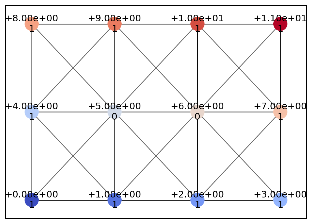
このままでは分かりづらいので,可視化用の関数を使ってグラフ構造を見てみます.入力データ構造の可視化には psiclone.visualization.draw_geometry を使います.

psiclone.visualization.draw_geometry(img)

このように,(3, 4) 形を持つ数値配列データがグラフ構造になっています.GrayscaleImage は画像データのような \(n \times m\) の数値データに特化した格子グラフをクラスになっています.

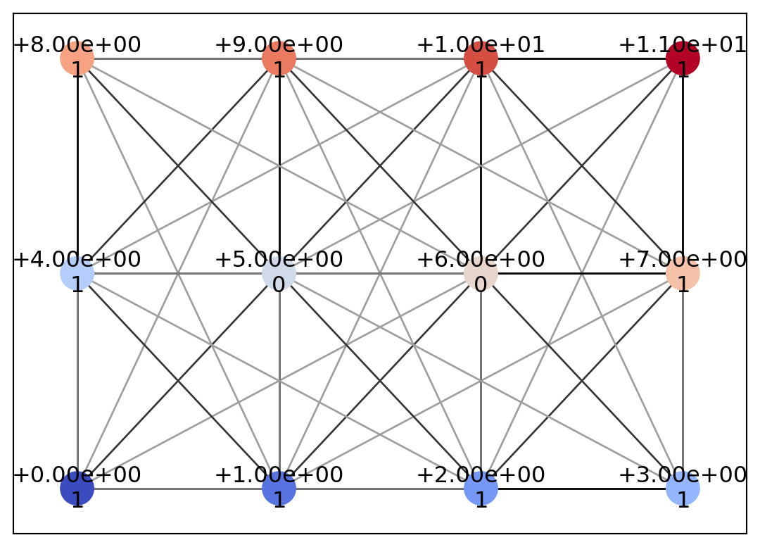
実は,第二引数 adjacency を与えることで別の隣接関係を使うこともできます.次のコードは八点近傍隣接関係の例です.

img = psiclone.data.GrayscaleImage(data, adjacency=psiclone.data.eight_points_adjacency())
psiclone.visualization.draw_geometry(img, edge_vmin=-2, edge_vmax=-1)

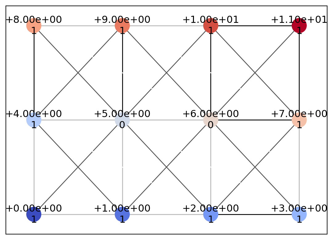
ノイズが極めて多いデータを扱う場合,前処理でノイズを除去しておくか,もしくはノイズのスケールに合わせて適切な隣接関係を用いることが有効です.多くの場合には上の例で用いたような八点近傍を用いるだけで十分な効果があります.次の例は,更に他の隣接関係を設定したものになります.

img = psiclone.data.GrayscaleImage(data, adjacency=psiclone.data.ball_adjacency(2, 2.5))
psiclone.visualization.draw_geometry(img, edge_vmin=-3, edge_vmax=-1)

入力データ Geometry

より一般に,座標と高さの値(と他にもいくつかのプロパティ)を持つグラフである psiclone.data.Geometry も入力データとして扱えます.実はこれは,GrayscaleImage から変換して得ることもできます.

geom = img.to_geometry()
geom.link_table
{Point(id=np.int64(0), level=np.int64(0), x=np.int64(0), y=np.int64(0), geotype=np.int64(1), order=np.float64(-2.498091544796509)): [<psiclone.data.graph.Edge at 0x7f5815c53980>,
  <psiclone.data.graph.Edge at 0x7f5815c57320>,
  <psiclone.data.graph.Edge at 0x7f5815ccdb20>,
  <psiclone.data.graph.Edge at 0x7f5815ccecf0>,
  <psiclone.data.graph.Edge at 0x7f5815ccd0d0>,
  <psiclone.data.graph.Edge at 0x7f5815ccede0>,
  <psiclone.data.graph.Edge at 0x7f5815ccfb60>],
 Point(id=np.int64(1), level=np.int64(1), x=np.int64(1), y=np.int64(0), geotype=np.int64(1), order=np.float64(-2.1587989303424644)): [<psiclone.data.graph.Edge at 0x7f5815c53980>,
  <psiclone.data.graph.Edge at 0x7f5815c54bc0>,
  <psiclone.data.graph.Edge at 0x7f5815b1dbb0>,
  <psiclone.data.graph.Edge at 0x7f5815b1ee10>,
  <psiclone.data.graph.Edge at 0x7f5815b1e660>,
  <psiclone.data.graph.Edge at 0x7f5815b1e960>,
  <psiclone.data.graph.Edge at 0x7f5815b1c6e0>,
  <psiclone.data.graph.Edge at 0x7f5815b1ce90>,
  <psiclone.data.graph.Edge at 0x7f5815b1f1d0>,
  <psiclone.data.graph.Edge at 0x7f5815b1e120>],
 Point(id=np.int64(2), level=np.int64(2), x=np.int64(2), y=np.int64(0), geotype=np.int64(1), order=np.float64(-1.5707963267948966)): [<psiclone.data.graph.Edge at 0x7f5815c57320>,
  <psiclone.data.graph.Edge at 0x7f5815c54bc0>,
  <psiclone.data.graph.Edge at 0x7f5815ccdbe0>,
  <psiclone.data.graph.Edge at 0x7f5815b1ee70>,
  <psiclone.data.graph.Edge at 0x7f5815b1c9b0>,
  <psiclone.data.graph.Edge at 0x7f5815cfb170>,
  <psiclone.data.graph.Edge at 0x7f5815cf8320>,
  <psiclone.data.graph.Edge at 0x7f5815cf9250>,
  <psiclone.data.graph.Edge at 0x7f5815cf8050>,
  <psiclone.data.graph.Edge at 0x7f5815cfab10>],
 Point(id=np.int64(3), level=np.int64(3), x=np.int64(3), y=np.int64(0), geotype=np.int64(1), order=np.float64(-0.982793723247329)): [<psiclone.data.graph.Edge at 0x7f5815b1dbb0>,
  <psiclone.data.graph.Edge at 0x7f5815ccdbe0>,
  <psiclone.data.graph.Edge at 0x7f5815b1e6c0>,
  <psiclone.data.graph.Edge at 0x7f5815cf9f10>,
  <psiclone.data.graph.Edge at 0x7f5815cf8530>,
  <psiclone.data.graph.Edge at 0x7f5815cf8f80>,
  <psiclone.data.graph.Edge at 0x7f5815cfa990>],
 Point(id=np.int64(4), level=np.int64(4), x=np.int64(0), y=np.int64(1), geotype=np.int64(1), order=np.float64(-2.896613990462929)): [<psiclone.data.graph.Edge at 0x7f5815ccdb20>,
  <psiclone.data.graph.Edge at 0x7f5815b1ee10>,
  <psiclone.data.graph.Edge at 0x7f5815b1ee70>,
  <psiclone.data.graph.Edge at 0x7f5815cf9820>,
  <psiclone.data.graph.Edge at 0x7f5815cf8680>,
  <psiclone.data.graph.Edge at 0x7f5815cfa2a0>,
  <psiclone.data.graph.Edge at 0x7f5815cf8c50>,
  <psiclone.data.graph.Edge at 0x7f5815cf9ac0>],
 Point(id=np.int64(5), level=np.int64(5), x=np.int64(1), y=np.int64(1), geotype=np.int64(0), order=np.float64(nan)): [<psiclone.data.graph.Edge at 0x7f5815ccecf0>,
  <psiclone.data.graph.Edge at 0x7f5815b1e660>,
  <psiclone.data.graph.Edge at 0x7f5815b1c9b0>,
  <psiclone.data.graph.Edge at 0x7f5815b1e6c0>,
  <psiclone.data.graph.Edge at 0x7f5815cf9820>,
  <psiclone.data.graph.Edge at 0x7f5815cfafc0>,
  <psiclone.data.graph.Edge at 0x7f5815cf8cb0>,
  <psiclone.data.graph.Edge at 0x7f5815cf94f0>,
  <psiclone.data.graph.Edge at 0x7f5815b2f440>,
  <psiclone.data.graph.Edge at 0x7f5815b2ef00>,
  <psiclone.data.graph.Edge at 0x7f5815b2f290>],
 Point(id=np.int64(6), level=np.int64(6), x=np.int64(2), y=np.int64(1), geotype=np.int64(0), order=np.float64(nan)): [<psiclone.data.graph.Edge at 0x7f5815ccd0d0>,
  <psiclone.data.graph.Edge at 0x7f5815b1e960>,
  <psiclone.data.graph.Edge at 0x7f5815cfb170>,
  <psiclone.data.graph.Edge at 0x7f5815cf9f10>,
  <psiclone.data.graph.Edge at 0x7f5815cf8680>,
  <psiclone.data.graph.Edge at 0x7f5815cfafc0>,
  <psiclone.data.graph.Edge at 0x7f5815cf8bc0>,
  <psiclone.data.graph.Edge at 0x7f5815b2f020>,
  <psiclone.data.graph.Edge at 0x7f5815b2ff80>,
  <psiclone.data.graph.Edge at 0x7f5815b2f830>,
  <psiclone.data.graph.Edge at 0x7f5815b2f080>],
 Point(id=np.int64(7), level=np.int64(7), x=np.int64(3), y=np.int64(1), geotype=np.int64(1), order=np.float64(-0.4636476090008061)): [<psiclone.data.graph.Edge at 0x7f5815b1c6e0>,
  <psiclone.data.graph.Edge at 0x7f5815cf8320>,
  <psiclone.data.graph.Edge at 0x7f5815cf8530>,
  <psiclone.data.graph.Edge at 0x7f5815cf8cb0>,
  <psiclone.data.graph.Edge at 0x7f5815cf8bc0>,
  <psiclone.data.graph.Edge at 0x7f5815b2ef30>,
  <psiclone.data.graph.Edge at 0x7f5815b2d130>,
  <psiclone.data.graph.Edge at 0x7f5815b2f740>],
 Point(id=np.int64(8), level=np.int64(8), x=np.int64(0), y=np.int64(2), geotype=np.int64(1), order=np.float64(2.896613990462929)): [<psiclone.data.graph.Edge at 0x7f5815ccede0>,
  <psiclone.data.graph.Edge at 0x7f5815b1ce90>,
  <psiclone.data.graph.Edge at 0x7f5815cfa2a0>,
  <psiclone.data.graph.Edge at 0x7f5815cf94f0>,
  <psiclone.data.graph.Edge at 0x7f5815b2f020>,
  <psiclone.data.graph.Edge at 0x7f5815b2ed80>,
  <psiclone.data.graph.Edge at 0x7f5815b2c500>],
 Point(id=np.int64(9), level=np.int64(9), x=np.int64(1), y=np.int64(2), geotype=np.int64(1), order=np.float64(2.677945044588987)): [<psiclone.data.graph.Edge at 0x7f5815ccfb60>,
  <psiclone.data.graph.Edge at 0x7f5815b1f1d0>,
  <psiclone.data.graph.Edge at 0x7f5815cf9250>,
  <psiclone.data.graph.Edge at 0x7f5815cf8c50>,
  <psiclone.data.graph.Edge at 0x7f5815b2f440>,
  <psiclone.data.graph.Edge at 0x7f5815b2ff80>,
  <psiclone.data.graph.Edge at 0x7f5815b2ef30>,
  <psiclone.data.graph.Edge at 0x7f5815b2ed80>,
  <psiclone.data.graph.Edge at 0x7f5815b2f800>,
  <psiclone.data.graph.Edge at 0x7f5815b2fd40>],
 Point(id=np.int64(10), level=np.int64(10), x=np.int64(2), y=np.int64(2), geotype=np.int64(1), order=np.float64(1.5707963267948966)): [<psiclone.data.graph.Edge at 0x7f5815b1e120>,
  <psiclone.data.graph.Edge at 0x7f5815cf8050>,
  <psiclone.data.graph.Edge at 0x7f5815cf8f80>,
  <psiclone.data.graph.Edge at 0x7f5815cf9ac0>,
  <psiclone.data.graph.Edge at 0x7f5815b2ef00>,
  <psiclone.data.graph.Edge at 0x7f5815b2f830>,
  <psiclone.data.graph.Edge at 0x7f5815b2d130>,
  <psiclone.data.graph.Edge at 0x7f5815b2c500>,
  <psiclone.data.graph.Edge at 0x7f5815b2f800>,
  <psiclone.data.graph.Edge at 0x7f5815b2f6b0>],
 Point(id=np.int64(11), level=np.int64(11), x=np.int64(3), y=np.int64(2), geotype=np.int64(1), order=np.float64(0.4636476090008061)): [<psiclone.data.graph.Edge at 0x7f5815cfab10>,
  <psiclone.data.graph.Edge at 0x7f5815cfa990>,
  <psiclone.data.graph.Edge at 0x7f5815b2f290>,
  <psiclone.data.graph.Edge at 0x7f5815b2f080>,
  <psiclone.data.graph.Edge at 0x7f5815b2f740>,
  <psiclone.data.graph.Edge at 0x7f5815b2fd40>,
  <psiclone.data.graph.Edge at 0x7f5815b2f6b0>]}
help(psiclone.data.geometry.Geometry)
Help on class Geometry in module psiclone.data.geometry:

class Geometry(psiclone.data.graph.Graph)
 |  A `Geometry` object models geometry of a collection of pixels with
 |  topological structure. An edge of `Geometry` has no properties,
 |  whereas a node of `Geometry` has the following properties.
 |  Note that this has nothing to do with geometric graphs in graph theory.
 |  In general, the edges are crossing and even not line segments.
 |
 |  Properties of Point
 |  -------------------
 |  id : int >= 0
 |  level : int, float
 |  x, y : int, float
 |  geotype : int >= 0
 |  order : int, float, optional
 |
 |  Note on the geotype property
 |  ----------------------------
 |  The geotype property may have any non-negative integer values.
 |  Geotype 0 is reserved for interior points.
 |  Geotype 1 is reserved for exterior points.
 |  Geotypes 2, 3, and so forth will be used for any other kind of geometric boundary points.
 |
 |  Method resolution order:
 |      Geometry
 |      psiclone.data.graph.Graph
 |      psiclone.data.abstract_graph.AbstractGraph
 |      builtins.object
 |
 |  Methods defined here:
 |
 |  __init__(self)
 |      Initialize self.  See help(type(self)) for accurate signature.
 |
 |  ----------------------------------------------------------------------
 |  Class methods defined here:
 |
 |  create_graph()
 |      Factory method of Graph.
 |
 |  create_node(*args, **kwgs)
 |      Factory method creating a Point instance.
 |
 |      Parameters
 |      ----------
 |      id : int >= 0
 |      level : int, float
 |      x, y : int, float
 |      geotype : int >= 0
 |      order : int, float, optional
 |
 |      Returns
 |      -------
 |      point : Point
 |          The point with specified properties.
 |
 |  ----------------------------------------------------------------------
 |  Static methods defined here:
 |
 |  modify_incompatible_id(geometry)
 |      Enforces node ids' uniqueness and sequential compatibility.
 |      The modification applies only to `Geometry` instance.
 |
 |      Parameters
 |      ----------
 |      geometry : `psiclone.data.Geometry`
 |          A `Geometry` object
 |
 |      Returns
 |      -------
 |      is_modified : bool
 |          True when incompatible ids are modified
 |
 |  ----------------------------------------------------------------------
 |  Data and other attributes defined here:
 |
 |  __abstractmethods__ = frozenset()
 |
 |  ----------------------------------------------------------------------
 |  Methods inherited from psiclone.data.graph.Graph:
 |
 |  __iadd__(self, other)
 |      Add an other graph into self.
 |
 |      Parameters
 |      ----------
 |      other : `psiclone.graph.Graph`
 |
 |  add_edge(self, node1, node2, *args, **kwgs)
 |      Create and add an edge linking node1 and node2.
 |
 |  add_node(self, *args, **kwgs)
 |      Create and add a node.
 |
 |  connected_components(self)
 |      Compute connected components.
 |
 |      Returns
 |      -------
 |      components : list
 |          A list of connected sub-graphs.
 |
 |  detach__edges(self, node)
 |      Make a node isolated so that each adjacent node is connected to a clone of the node.
 |
 |      Parameters
 |      ----------
 |      node : `psiclone.graph.Node`
 |          A node to be detached.
 |
 |      Returns
 |      -------
 |      new__nodes : list
 |          A list of __nodes cloned from the original node.
 |
 |  find_walk(self, src, dest)
 |      Find a path from `src` to `dest`.
 |
 |      Parameters
 |      ----------
 |      src, dest : `psiclone.graph.Node`
 |          Source and destination nodes.
 |
 |      Returns
 |      -------
 |      walk : list, None
 |          A list of __edges that realizes the found path.
 |          None is returned if not found.
 |
 |  invert_branch(self, branch1, branch2, midnode)
 |      Try to invert branch operation. Note that `midnode` is not removed.
 |
 |      Parameters
 |      ----------
 |      branch1, branch2 : `psiclone.graph.Edge`
 |          Edges connecting a common `midnode`.
 |
 |      midnode : `psiclone.graph.Node`
 |          A common node connected with `branch1` and `branch2`.
 |
 |      Returns
 |      -------
 |      edge : `psiclone.graph.Edge`
 |          An edge recovered from `branch1` and `branch2`.
 |
 |  reconnect(self, edge, old_node, new_node)
 |      Replace a connected `old_node` by `new_node` in `edge`.
 |
 |      Parameters
 |      ----------
 |      edge : `psiclone.graph.Edge`
 |          An edge to be reconnected.
 |
 |      old_node, new_node : `psiclone.graph.Node`
 |          Nodes to be replaced.
 |
 |  reduce(self, edge, needless_node)
 |      Reduce a node in the direction of an edge.
 |
 |      Parameters
 |      ----------
 |      edge : `psiclone.graph.Edge`
 |          An edge to be reduced.
 |
 |      needless_node : `psiclone.graph.Node`
 |          A node to be removed.
 |
 |  register_edge(self, edge)
 |      Register the edge instance.
 |
 |  register_node(self, node)
 |      Register the node instance.
 |
 |  remove_edge(self, edge)
 |      Remove the edge.
 |
 |  remove_node(self, node)
 |      Remove the node.
 |
 |  subgraph(self, nodes, edges=None)
 |      Create a sub-graph made of given nodes.
 |
 |      Parameters
 |      ----------
 |      nodes : list
 |          A list of subgraph nodes. Not copied.
 |
 |      edges : list, optional
 |          A list of subgraph edges. Not copied.
 |          All the edges linking given nodes are used if omitted.
 |
 |      Returns
 |      -------
 |      other : `psiclone.graph.Graph`
 |          A graph made of given nodes.
 |
 |  walk_deeply(self, initial_node, fun)
 |      Walk from `initial_node` and apply `fun` to each node in a deep recursion.
 |
 |      Parameters
 |      ----------
 |      initial_node : `psiclone.graph.Node`
 |          A first node to visit.
 |
 |      fun : callable
 |          A function with the signature `fun(node, n)` applied to each node.
 |
 |          Parameters
 |          ----------
 |          node : `psiclone.graph.Node`
 |              Every node path-connected with `initial_node`.
 |
 |          n : int >= 0
 |              Recursion depth, or a path length, from `initial_node`.
 |              Note that this does not coincide with the shortest path length in general.
 |
 |  ----------------------------------------------------------------------
 |  Class methods inherited from psiclone.data.graph.Graph:
 |
 |  create_edge(node1, node2, *args, **kwgs)
 |      Factory method creating an Edge instance.
 |
 |  ----------------------------------------------------------------------
 |  Readonly properties inherited from psiclone.data.graph.Graph:
 |
 |  edges
 |
 |  link_table
 |
 |  nodes
 |
 |  ----------------------------------------------------------------------
 |  Methods inherited from psiclone.data.abstract_graph.AbstractGraph:
 |
 |  to_network(self)
 |
 |  ----------------------------------------------------------------------
 |  Data descriptors inherited from psiclone.data.abstract_graph.AbstractGraph:
 |
 |  __dict__
 |      dictionary for instance variables
 |
 |  __weakref__
 |      list of weak references to the object

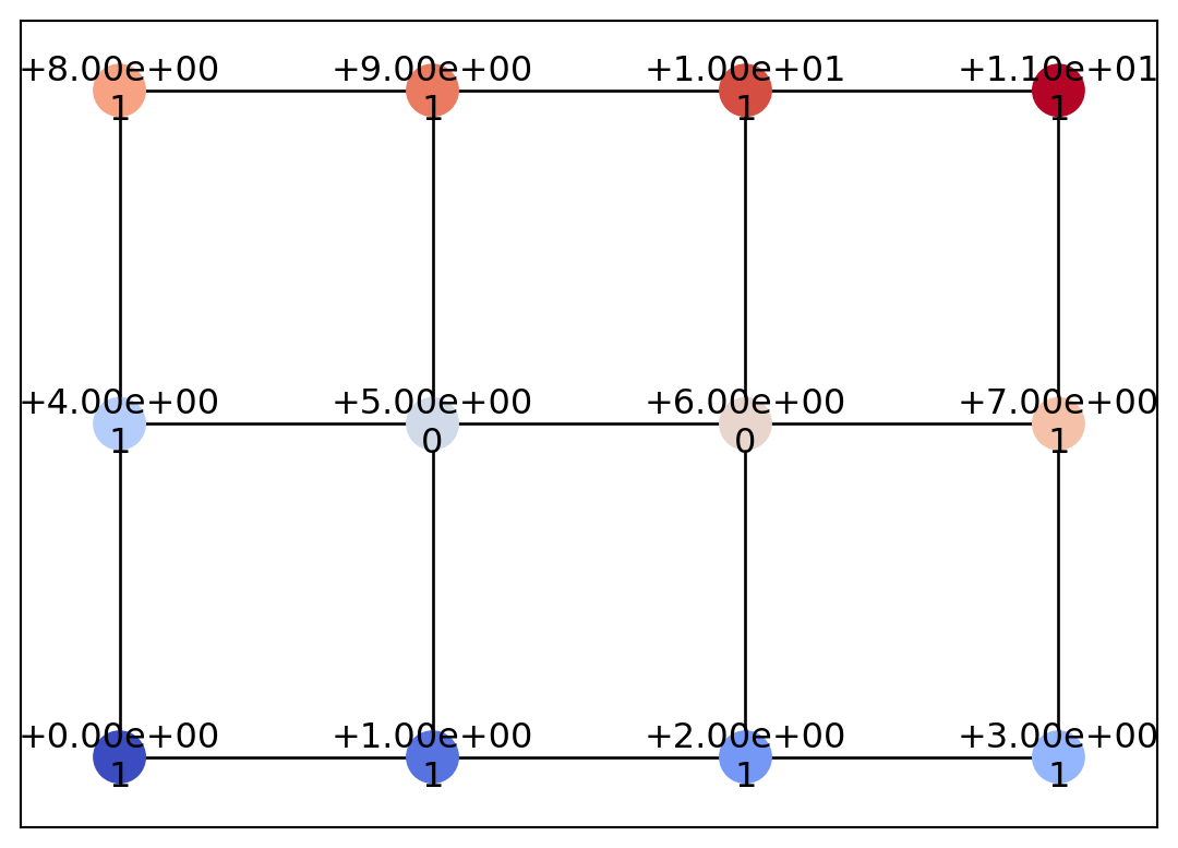
やはり内部データを見ても分かりづらいので,Geometry オブジェクトを可視化してみましょう.前の例と同様に draw_geometry 関数を使います.

psiclone.visualization.draw_geometry(geom)

最初と全く同じ格子グラフになっていることが分かります.

Geometryを直接作る

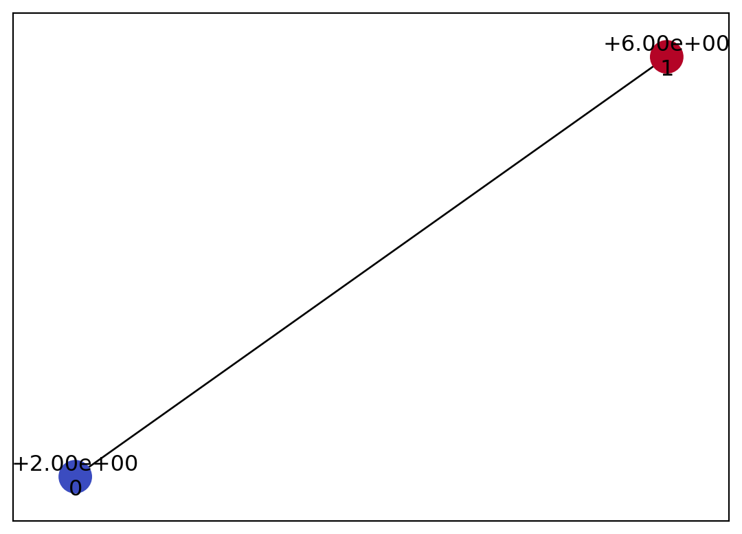
簡単な Geometry オブジェクトをスクラッチで作ってみましょう.このチュートリアルでは,複雑な Geometry オブジェクトの作成方法等については詳しくは説明しません.基本的には,add_node で頂点を,add_edge で辺を追加していくことで任意の幾何形状の離散化を表現します.

geom = psiclone.data.geometry.Geometry()
n1 = geom.add_node(id=0, level=2, x=3, y=4, geotype=psiclone.data.Geotype.INTERIOR)  # , order)
n2 = geom.add_node(id=1, level=6, x=7, y=8, geotype=psiclone.data.Geotype.EXTERIOR)  # , order)
geom.add_edge(n1, n2)
<psiclone.data.graph.Edge at 0x7f5815cf93d0>
psiclone.visualization.draw_geometry(geom)

レーブグラフ

さて,いよいよ入力データを解析プログラムにかけていきます.流線トポロジー解析に入る前に,流線トポロジー解析において重要な役割を持つレーブグラフについてまずは見ておきましょう.

レーブグラフは等高線のトポロジカルな構造をグラフを用いて要約したものです.psiclone.reeb.get_reeb_graph 関数を用いて計算することができます.と言っても,ここまでで扱ってきた単純な入力データ例ではトポロジカルに自明な構造しかないため結果も自明なものになります.

reeb = psiclone.reeb.get_reeb_graph(img)
networkx.draw(reeb.to_network())

非自明な簡単な例を作ってみます.

y, x = numpy.mgrid[-2:3, -2:3]
f = x * x - y * y
f
array([[ 0, -3, -4, -3,  0],
       [ 3,  0, -1,  0,  3],
       [ 4,  1,  0,  1,  4],
       [ 3,  0, -1,  0,  3],
       [ 0, -3, -4, -3,  0]])
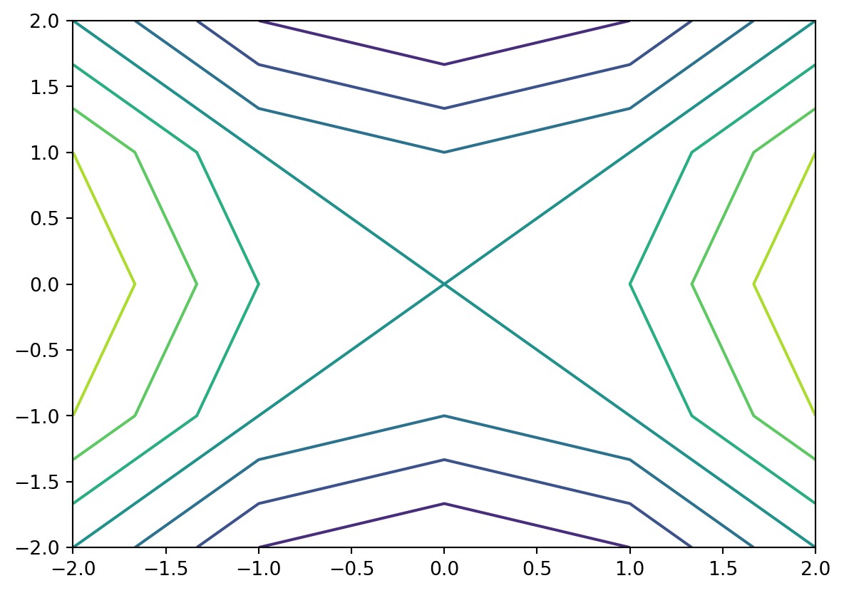
plt.contour(x, y, f)

見ての通り,この例は \(f(x,y) = x^2 - y^2\) という高さ関数の \((5, 5)\) 格子サンプルです.もちろん,この関数は原点に鞍点を持ち,高さ \(f = 0\) を境に等高線のトポロジーが変化します.では,レーブグラフを見てみましょう.

plt.figure(figsize=(8, 8))

img = psiclone.data.GrayscaleImage(f)
reeb = psiclone.reeb.get_reeb_graph(img)
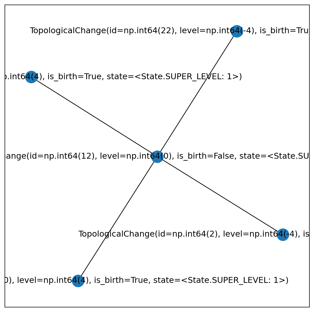
networkx.draw_networkx(reeb.to_network())

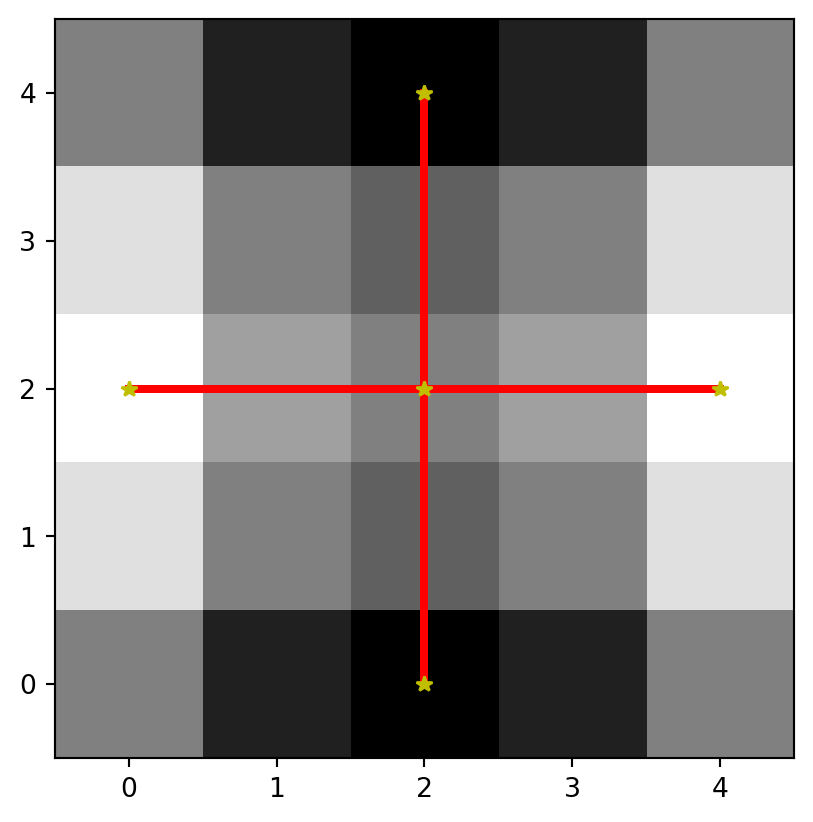
等高線は原点を中心に四種類に分かれていますから,レーブグラフも高さ \(0\) の対応するノードが次数 \(4\) になっており,四本のエッジへと枝分かれしています.psiclone.visualization.draw_graph_markers を使うと元のデータでの位相変化点がどこにあるのか分かります.

plt.imshow(f, origin="lower", cmap="gray")
psiclone.visualization.draw_graph_markers(graph=reeb, geometry=img, lw=3, edge_color="r-")


演習問題:好きな式で等高線図を作りレーブグラフを計算してみよう

# グリッド変数を numpy.mgrid[y0:y1:y分割数j, x0:x1:x分割数j] で用意します.
# ただし,分割数は虚数単位の整数倍で指定します:
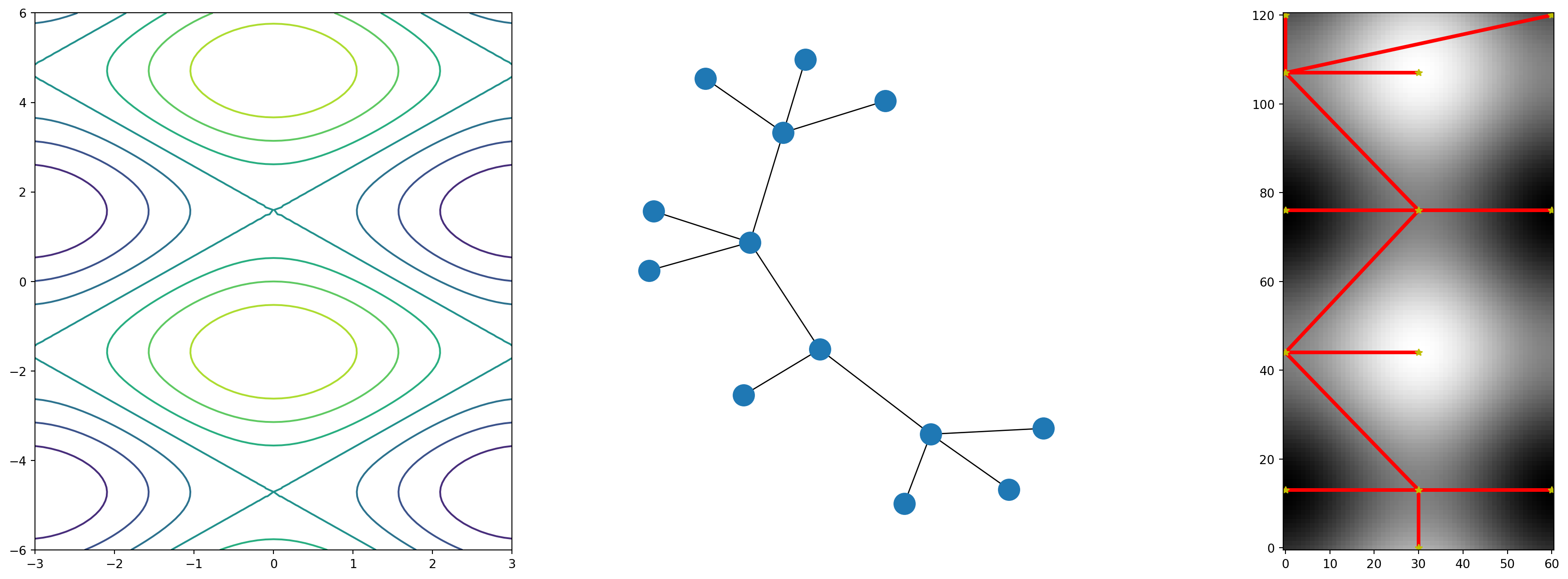
y, x = numpy.mgrid[-6:6:121j, -3:3:61j]
# 好きな式を入れてみましょう.
f = numpy.cos(x) - numpy.sin(y)
# GrayscaleImage に変換し,Reeb グラフを計算します.
img = psiclone.data.GrayscaleImage(f)
reeb = psiclone.reeb.get_reeb_graph(img)

fig = plt.figure(figsize=(24, 8))
fig.add_subplot(1, 3, 1)
plt.contour(x, y, f)

fig.add_subplot(1, 3, 2)
networkx.draw(reeb.to_network())

fig.add_subplot(1, 3, 3)
plt.imshow(f, origin="lower", cmap="gray")
psiclone.visualization.draw_graph_markers(graph=reeb, geometry=img, lw=3, edge_color="r-")


流れデータの解析 (TFDA)

一様流れの場合

中心に障害物が一つ置かれている問題設定で (x, y, z) が複数並ぶ入力データを読み込み,一様流れの COT 表現に変換します.

import psiclone.visualization as vis
from psiclone.psi2tree import Psi2tree
from psiclone.util.convert import convert_array_to_geometry

ここまではモジュールをただの import 文で読み込んで来ましたが,よく使うものは from import 文で直接読み込むと便利です.ここでは,Psi2treeconvert_array_to_geometry を用いて,流線トポロジー解析を行います.まずは,テストデータを作成します.

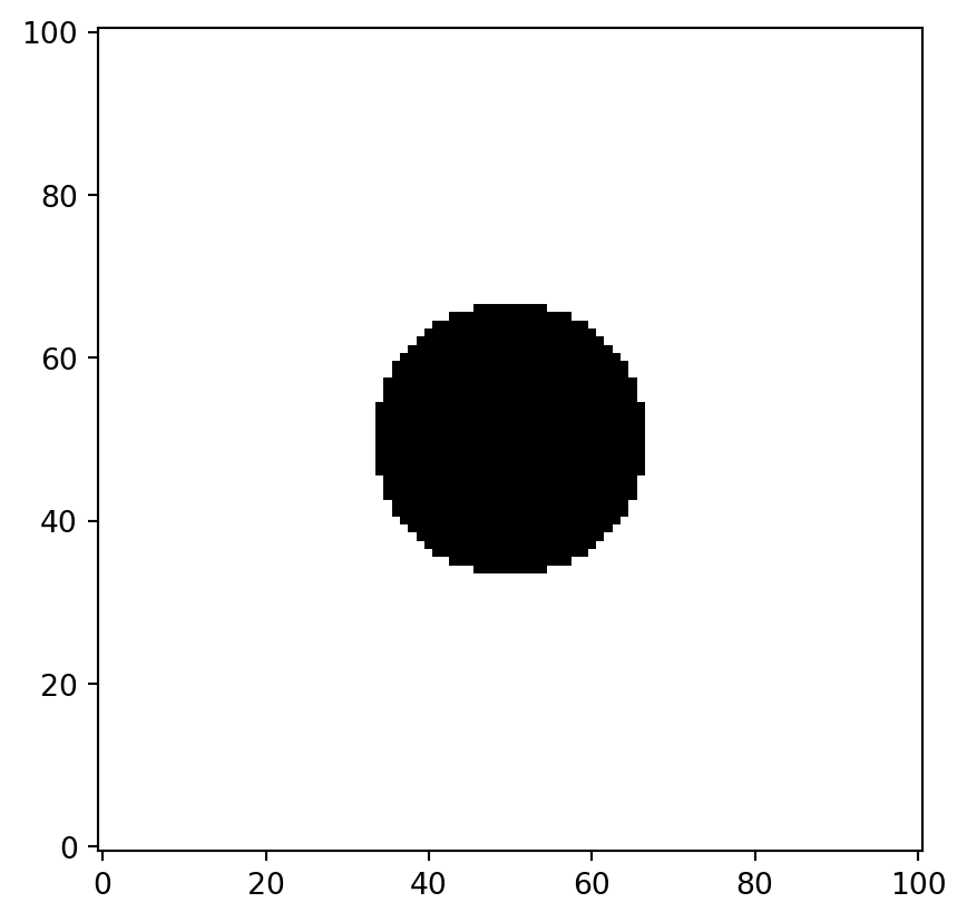
y, x = numpy.mgrid[-3:3:101j, -3:3:101j]
z = x + y * 1j
flow_domain = numpy.abs(z) >= 1.0
obstacle_domain = ~flow_domain  # 否定

plt.imshow(flow_domain, cmap="gray", origin="lower")

mesh grid を作成して,虚数単位 1j を用いて複素変数 \(z = x + y\sqrt{-1}\) を用意しました.円形の障害物が中央にある流れ領域として \(\{z : \left|z\right| \ge 1\}\) を考えています.

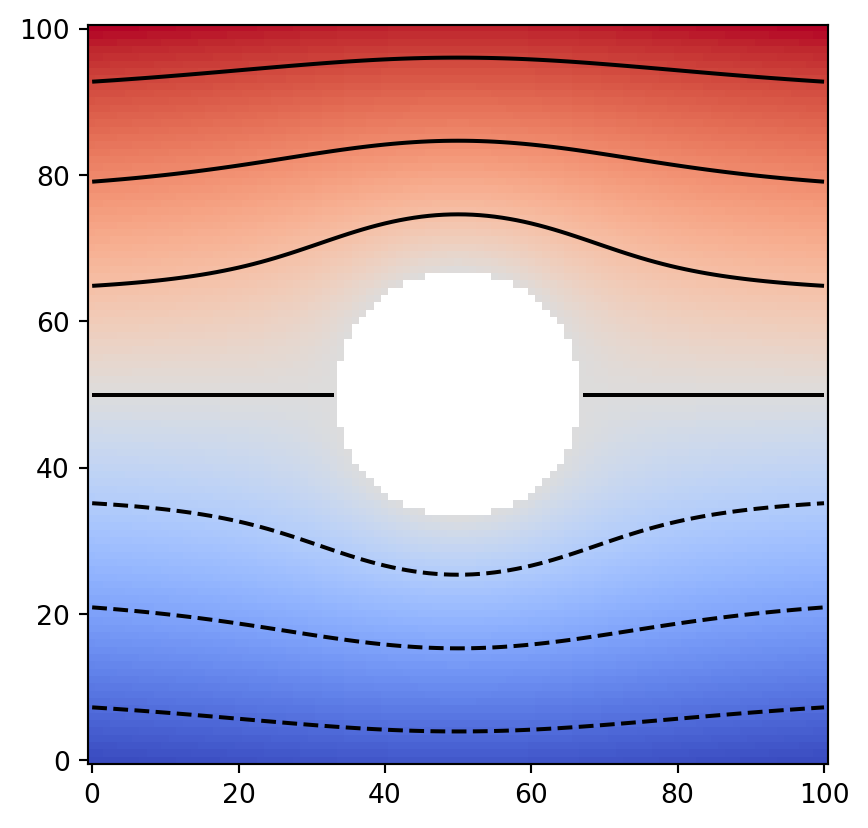
その上のデータを表現するには,numpy.ma.masked_array を利用すると便利です.これは,データ欠損領域をマスクを用いて指定できる特殊な配列です.データ欠損領域がある以外は,通常の numpy.ndarray と同様に扱うことが可能です.さて,複素変数 \(z\)masked_array を用いて,次のように流線関数を用意します.

z = numpy.ma.masked_array(z, obstacle_domain)
W = z + 1.0 / z
data = numpy.imag(W)
plt.imshow(data, cmap="coolwarm", origin="lower")
plt.contour(data, colors="k")

これで,円形障害物の周りを流れる一様流のテストデータが作れました.これを Geometry に変換していきます.

table = numpy.ma.masked_array([x, y, data]).reshape((3, -1)).T
table.shape
(10201, 3)

障害物のある一様流の設定で Geometry を構成するユーティリティ関数 psiclone.util.convert.convert_array_to_geometry を用います.そのために,まず x, y, f(x,y)が並んだ \(N \times 3\) の表データをマスクした配列として用意しました.(マスク配列の代わりに,nan を用いてデータ欠損領域を表現したデータや,単純にデータ欠損領域のエントリーを含まない表データでも構いません.)

この関数には,色々なオプション引数がありますが,ここでは障害物を指定する引数 obstacles に一つの障害物の座標だけを指定します.各障害物ごとに代表点の座標を一つだけ指定すれば十分です.この例では原点を指定しています.

geom = convert_array_to_geometry(table, obstacles=[(0, 0)])
geom, len(geom.nodes), len(geom.edges)
(<psiclone.data.geometry.Geometry at 0x7f580b543830>, 9325, 18476)

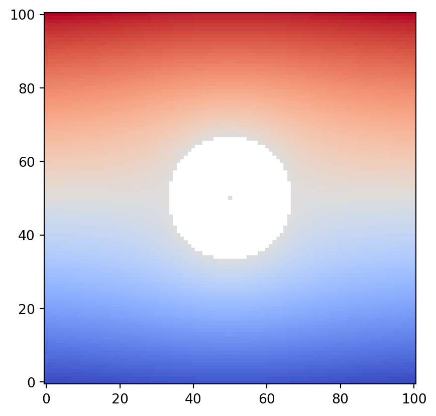
このように構成した geom が上と同じデータになっているか,確認してみましょう.ようやく入力データが用意できました.ここまで来れば,次はいよいよ TFDA のステップです!

vis.draw_geometry(geom, bitmap=True)

入力データの COT 表現への変換:psiclone.psi2tree.Psi2tree

さて,Geometry を入力データにとって,partially Cyclically Ordered rooted Tree (COT) 表現の計算を行います.これは,psiclone.psi2tree.Psi2tree クラスを使います.この名前は,流線関数 psi (\(\psi\)) to (2) tree の略になっています.

psi2tree = Psi2tree(geom, threshold=0.0)
psi2tree.compute()

計算は compute メソッドで実行します.入力データによっては,ここで非常に時間がかかるために,適切なノイズ除去閾値 threshold を設定するなどしなければならない場合があります.また,あまりに大きすぎる入力データのトポロジー計算は時間がかかるため,入力データサイズ自体をうまく resize して減らしてやることも有効です.

計算が終わったら,結果を get_tree メソッドで取得します.get_tree で取得できる木構造データを,さらに convert メソッドを用いて,人が読みやすい形式に変換します.

from psiclone.cot import to_str

psi2tree.get_tree().convert(to_str)
'a0(a2(L+,L-))'

COT 表現の出力形式

convert メソッドに以下のいずれかを与えることで COT 表現を様々な出力形式へと変換できます. * psiclone.cot.to_str * psiclone.cot.to_short_str * psiclone.cot.to_tex * psiclone.cot.to_short_tex

to_(short_)str はギリシャ文字などを含まない簡易 ASCII フォーマットへ変換し,to_(short_)tex は TeX 形式で正しい添字やギリシャ文字によるラベル付けをした形式へ変換します.short_ 版は人が読みやすい省略形式で,情報を失わない範囲で冗長な記号を省略します.convert に渡す関数を変えることで再帰的な変換をカスタマイズすることも可能です.

from IPython.display import Math, display

from psiclone.cot import to_short_str, to_short_tex

cot_tree = psi2tree.get_tree()
print(cot_tree.convert(to_short_str))
print(cot_tree.convert(to_short_tex))
display(Math(cot_tree.convert(to_short_tex)))
a0(a2)
a_\emptyset(a_2)

\(\displaystyle a_\emptyset(a_2)\)

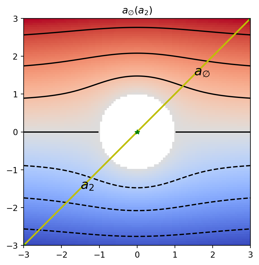
入力データ・等高線図・レーブグラフ・COT表現を重ねて描いてみましょう.

plt.title(f"${psi2tree.get_tree().convert(to_short_tex)}$")
plt.imshow(data, cmap="coolwarm", origin="lower", extent=[numpy.amin(x), numpy.amax(x), numpy.amin(y), numpy.amax(y)])
plt.contour(x, y, data, colors="k")
vis.draw_graph_markers(psi2tree, lw=2, edge_color="y-", node_color="g*")
vis.draw_COT_labels(psi2tree, fontsize=16)


演習問題:式を少し摂動してみて計算結果がどうなるか見てみましょう

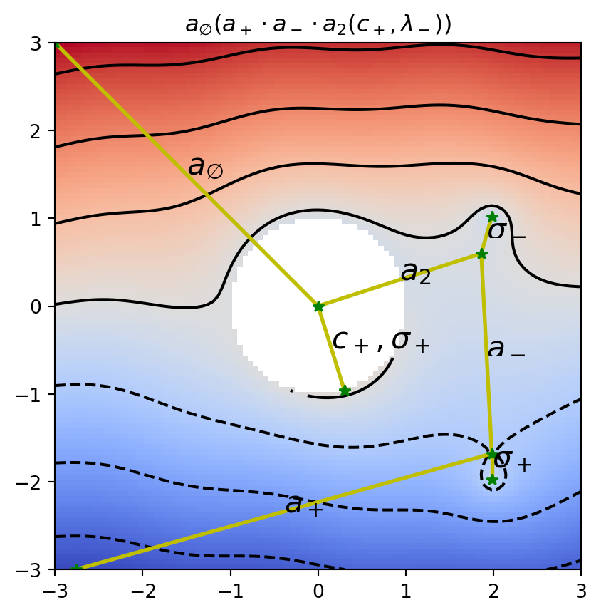
上の例の一様流に,適当な摂動を加えてみて,計算結果を見てみましょう.

ただし,あまりに大きな摂動を加え過ぎると,ノイズが除去しきれずに,レーブグラフや COT 表現の計算に失敗してしまう可能性があります.ここでは threshold=1.0e-1 をノイズ除去の閾値にしていますから,面白い構造はこれより大きなスケールに,またノイズはこれより小さなスケールになっていなければなりません.

y, x = numpy.mgrid[-3:3:101j, -3:3:101j]
z = x + y * 1j
flow_domain = numpy.abs(z) >= 1.0
obstacle_domain = ~flow_domain

z = numpy.ma.masked_array(z, obstacle_domain)
W = z + 1.0 / z
perturbation = 4.0e-2 * numpy.sin(numpy.pi * x)
perturbation += 0.3 * numpy.log(numpy.abs(z - (2.0 + 1.0j)))
perturbation -= 0.3 * numpy.log(numpy.abs(z - (2.0 - 2.0j)))
data = numpy.imag(W) + flow_domain * perturbation

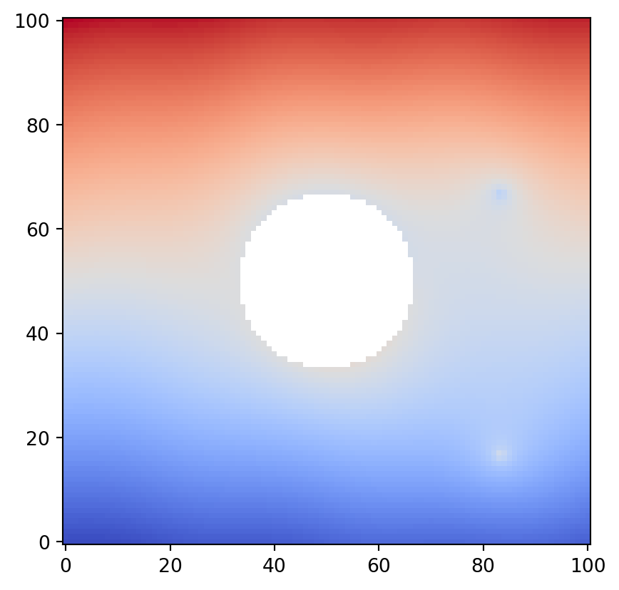
plt.imshow(data, origin="lower", cmap="coolwarm")
/tmp/ipykernel_3850/2062294558.py:9: RuntimeWarning:

divide by zero encountered in log

/tmp/ipykernel_3850/2062294558.py:10: RuntimeWarning:

divide by zero encountered in log

table = numpy.ma.masked_array([x, y, data]).reshape((3, -1)).T
geom = convert_array_to_geometry(table, obstacles=[(0, 0)])
psi2tree = Psi2tree(geom, threshold=1.0e-1)

cot_tree = None
cot_tex = "\\rm Error"
try:
    psi2tree.compute()
    cot_tree = psi2tree.get_tree()
    cot_tex = cot_tree.convert(to_short_tex)
except Exception as e:
    print(e)

plt.title(f"${cot_tex}$")
plt.imshow(data, cmap="coolwarm", origin="lower", extent=[numpy.amin(x), numpy.amax(x), numpy.amin(y), numpy.amax(y)])
plt.contour(x, y, data, colors="k")
vis.draw_graph_markers(psi2tree, lw=2, edge_color="y-", node_color="g*")
if cot_tree is not None:
    vis.draw_COT_labels(psi2tree, fontsize=16)

分割の可視化

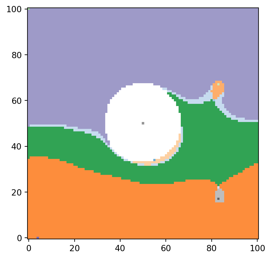
数学的には,レーブグラフは同値関係による商空間として定まります.psiclone で用いられているアルゴリズムでも,同値関係に基づく空間の分割が得られます.

分割を可視化するには,psiclone.visualization.draw_partition 関数が便利です.これを見ると,レーブグラフを通して psiclone がどのように流線トポロジーを把握しているかがなんとなく分かります.

vis.draw_partition(psi2tree, bitmap=True, discrete=True, cmap="tab20c")