2次元メッシュ（非構造格子）データの取り扱い

psiclone はメッシュ（非構造格子）データの読み込みには対応していませんが，Geometry オブジェクトを直接構成すれば任意の非構造格子データに対しても計算が可能です．具体的には，Geometry オブジェクトにノードとエッジを追加して，これを Psi2tree の入力データとして用いればよいです．以下では，この方法の一連の流れを解説していきます．

import numpy

from psiclone.data import Geometry, GrayscaleImage
from psiclone.visualization import draw_geometry

まず GrayscaleImage を Geometry に変換して，このオブジェクトがどのようなデータ構造を保持しているか確認してみましょう．

img = GrayscaleImage(numpy.arange(12).reshape((3, 4)))
geom = img.to_geometry()
geom.nodes

[Point(id=np.int64(0), level=np.int64(0), x=np.int64(0), y=np.int64(0), geotype=np.int64(1), order=np.float64(-2.498091544796509)),
 Point(id=np.int64(1), level=np.int64(1), x=np.int64(1), y=np.int64(0), geotype=np.int64(1), order=np.float64(-2.1587989303424644)),
 Point(id=np.int64(2), level=np.int64(2), x=np.int64(2), y=np.int64(0), geotype=np.int64(1), order=np.float64(-1.5707963267948966)),
 Point(id=np.int64(3), level=np.int64(3), x=np.int64(3), y=np.int64(0), geotype=np.int64(1), order=np.float64(-0.982793723247329)),
 Point(id=np.int64(4), level=np.int64(4), x=np.int64(0), y=np.int64(1), geotype=np.int64(1), order=np.float64(-2.896613990462929)),
 Point(id=np.int64(5), level=np.int64(5), x=np.int64(1), y=np.int64(1), geotype=np.int64(0), order=np.float64(nan)),
 Point(id=np.int64(6), level=np.int64(6), x=np.int64(2), y=np.int64(1), geotype=np.int64(0), order=np.float64(nan)),
 Point(id=np.int64(7), level=np.int64(7), x=np.int64(3), y=np.int64(1), geotype=np.int64(1), order=np.float64(-0.4636476090008061)),
 Point(id=np.int64(8), level=np.int64(8), x=np.int64(0), y=np.int64(2), geotype=np.int64(1), order=np.float64(2.896613990462929)),
 Point(id=np.int64(9), level=np.int64(9), x=np.int64(1), y=np.int64(2), geotype=np.int64(1), order=np.float64(2.677945044588987)),
 Point(id=np.int64(10), level=np.int64(10), x=np.int64(2), y=np.int64(2), geotype=np.int64(1), order=np.float64(1.5707963267948966)),
 Point(id=np.int64(11), level=np.int64(11), x=np.int64(3), y=np.int64(2), geotype=np.int64(1), order=np.float64(0.4636476090008061))]

draw_geometry(geom)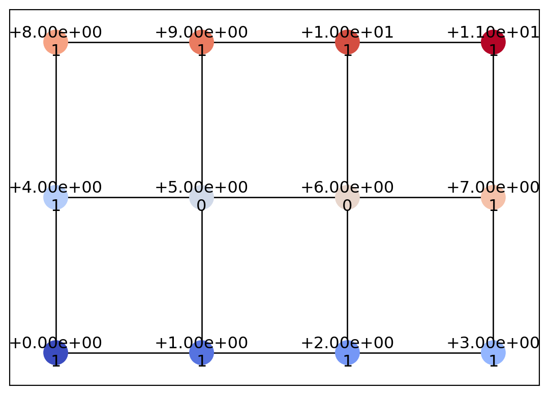

このように，GrayscaleImage オブジェクト（から変換して得た Geomery オブジェクト）はフォン・ノイマン近傍（四方向接続）の格子グラフによって構成されていることが分かります．ここに，「斜め」のエッジを追加してみます．

for i in range(2):
    for j in range(3):
        idx = 4 * i + j
        geom.add_edge(geom.nodes[idx], geom.nodes[idx + 5])

draw_geometry(geom, edge_color="k")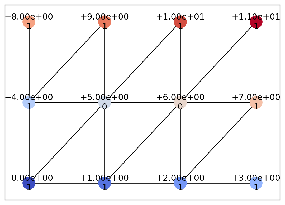

このように，三角形メッシュを作ることができました．psiclone の COT 表現計算アルゴリズムは，グラフ上に定義されたスカラー値と，グラフの隣接構造に基づいています．したがって，このように同じ座標上で定義されたスカラーデータであっても，グラフの隣接構造が異なれば一般には計算結果も異なる可能性があることに注意してください．

また，Geometry はただのグラフ構造データですから，次の例のように三角形以外の構造を持っていても構いません．

from psiclone.data import Geotype

ex_node = geom.add_node(id=12, x=4.5, y=1, level=-1, geotype=Geotype.EXTERIOR)
geom.add_edge(ex_node, geom.nodes[3])
geom.add_edge(ex_node, geom.nodes[11])
draw_geometry(geom, edge_color="k")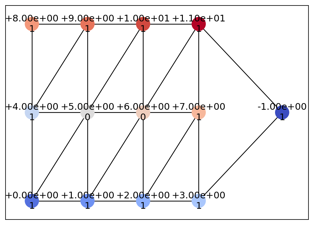

もう少し実用的に，メッシュデータから COT 表現を計算する例を見てみましょう．ここでは，scipy.spatial.Delaunay を使って，ドロネー三角形分割の上にデータを定義してみます．Delaunay() の詳細についてはSciPy のドキュメントを参照してください．

import matplotlib.pyplot as plt
from scipy.spatial import Delaunay

# Generate Delauny triangulation from random points
num_points = 20
points = numpy.random.rand(num_points, 2)
tri = Delaunay(points)

plt.triplot(points[:, 0], points[:, 1], tri.simplices)
plt.plot(points[:, 0], points[:, 1], "o")
plt.show()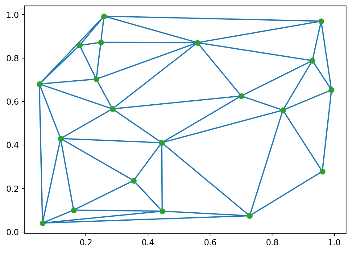

ランダム生成した点群 points から，scipy.spatial.Delaunay() 関数を用いてドロネー三角形分割を生成しました．結果はオブジェクト tri に格納されています．三角形（単体 = simplex）のデータは tri.simplices に格納されています．各 simplex は，ノード番号の三つ組になっています．これらをもとに，ノードとエッジを空の Geometry オブジェクトに追加していきます．

Geometry の各ノードにいくつかの付加情報が必要です．geotype 属性は，入力空間の内部ノードには Geotype.INTERIOR を，入力空間の境界（外部）ノードには Geotype.EXTERIOR を割り当てます．他にも，データの境界条件によっては order 属性も必要となる場合があります．なお，入力空間が単連結でなく多重連結空間である場合には，geotype 属性にさらに他の値を割り振る必要があります（詳しくは, psiclone.util.mcdomain を用いて有界流れを解析する場合を参照してください）．この例では，geotype 属性だけ tri.convex_hull に基づいて設定しておきましょう．

mesh = Geometry()


def f(x, y):
    return x**2 + numpy.cos(8 * y)


boundary_indices = set(numpy.unique(tri.convex_hull))

for i, (x, y) in enumerate(tri.points):
    geotype = Geotype.EXTERIOR if i in boundary_indices else Geotype.INTERIOR
    mesh.add_node(id=i, x=x, y=y, level=f(x, y), geotype=geotype)

has_edge = numpy.zeros((num_points, num_points), dtype="bool")
for simplex in tri.simplices:
    for a, b in zip(simplex, numpy.roll(simplex, 1), strict=False):
        if has_edge[a, b]:
            continue
        mesh.add_edge(mesh.nodes[a], mesh.nodes[b])
        has_edge[a, b] = has_edge[b, a] = True

draw_geometry(mesh, edge_color="k")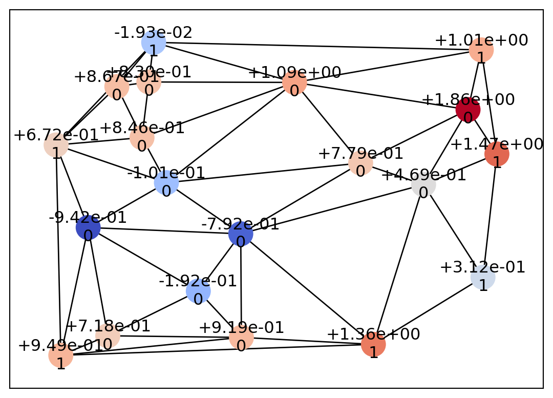

これで入力空間データの設定が完了しました．あとは Psi2tree でこの入力データを処理します．

from psiclone.cot import to_str
from psiclone.psi2tree import Psi2tree

psi2tree = Psi2tree(geom, threshold=0.0)
psi2tree.compute()
psi2tree.get_tree().convert(to_str)

'a0(L~)'

無事，COT 表現に変換できました．

Other Formats