import matplotlib.pyplot as plt
import numpy

import psiclone.visualization as vis
from psiclone.psi2tree import Psi2treeVisualization Module psiclone.visualization
Here we introduce how to use the functions provided by the visualization module psiclone.visualization.
The main functions of this module are as follows:
draw_COT_labels()– Draws only the COT labels near each edge of the Reeb graphdraw_barcode()– Draws barcode diagrams for persistent homology and the Reeb graphdraw_bitmap()– Draws an input data space compatible with theGrayscaleImagetypedraw_contour()– Draws contour plotsdraw_geometry()– Draws an input data space of typeGeometrydraw_graph()– Draws only the Reeb graph (via NetworkX)draw_graph_markers()– Draws Reeb graph nodes and edges in the coordinates of the input data spacedraw_partition()– Draws the partition diagram corresponding to the Reeb graphget_COT_constructions()– Retrieves recursive COT constructions and corresponding partition informationget_barcode_data()– Retrieves barcode data (corresponding todraw_barcode())get_graph_markers_data()– Retrieves Reeb graph coordinate data (corresponding todraw_graph_markers())get_partition_data()– Retrieves partition diagram data (corresponding todraw_partition())
Many of the draw_***() visualization functions are provided primarily for simple experimentation and tutorial purposes.
For advanced, specialized, or production-level visualization, it is better to not use these convenience functions.
If you require advanced visualization, it is recommended to use libraries such as Matplotlib directly.
For example, the visualization module always draws on the current Axes (matplotlib.pyplot.gca()).
If you need finer customization, such as drawing on a specific Axes, you will need to implement your own visualization code. In such cases, utilize the get_***() functions to obtain the necessary drawing data.
Preparing the Input Data
First, we prepare the input data space.
We construct the example using the same method as in the tutorial.
from psiclone.util.convert import convert_array_to_geometry

x0, x1, y0, y1 = -3.0, 3.0, -2.5, 2.5
x, y = numpy.mgrid[x0:x1:15j, y0:y1:15j]
z = x + y * 1j
flow_domain = numpy.abs(z) >= 1.0
obstacle_domain = ~flow_domain

z = numpy.ma.masked_array(z, obstacle_domain)
W = z + 1.0 / z
data = numpy.imag(W)

table = numpy.ma.masked_array([x, y, data]).reshape((3, -1)).T
geom = convert_array_to_geometry(table, obstacles=[(0, 0)], int_grid=False)
geom
<psiclone.data.geometry.Geometry at 0x7f3a51efd400>We also compute the COT representation in advance.
from psiclone.cot import to_str

psi2tree = Psi2tree(geom, threshold=1.0e-2)
psi2tree.compute()
psi2tree.get_tree().convert(to_str)'a0(a2(L+,L-))'Basic Drawing Functions
psiclone.visualization.draw_bitmap()
The draw_bitmap() function draws the height (level) of an input data space with integer coordinates compatible with the GrayscaleImage type.
vis.draw_bitmap(geom)
In psiclone, the origin of the drawing coordinates is consistently set at the lower left.
This is because psiclone is a library for analyzing streamline diagrams.
It follows the default coordinate convention of matplotlib.pyplot.contour and standard mathematical practice.
psiclone.visualization.draw_geometry()
The draw_geometry() function draws a general input data space of type Geometry.
If bitmap=True is specified, it uses draw_bitmap().
If bitmap=False, it uses draw_networkx().
The same bitmap option is available in several of the drawing functions introduced below.
vis.draw_geometry(geom, bitmap=True)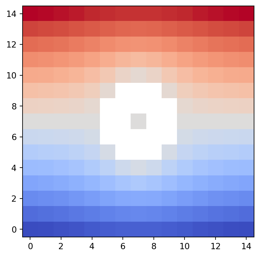
In general, using bitmap=False (NetworkX) for large datasets is not recommended. Since the current input data space example is sufficiently coarse, we intentionally specify bitmap=False by increasing figsize and dpi.
plt.figure(figsize=(7, 5), dpi=150)
vis.draw_geometry(geom, bitmap=False)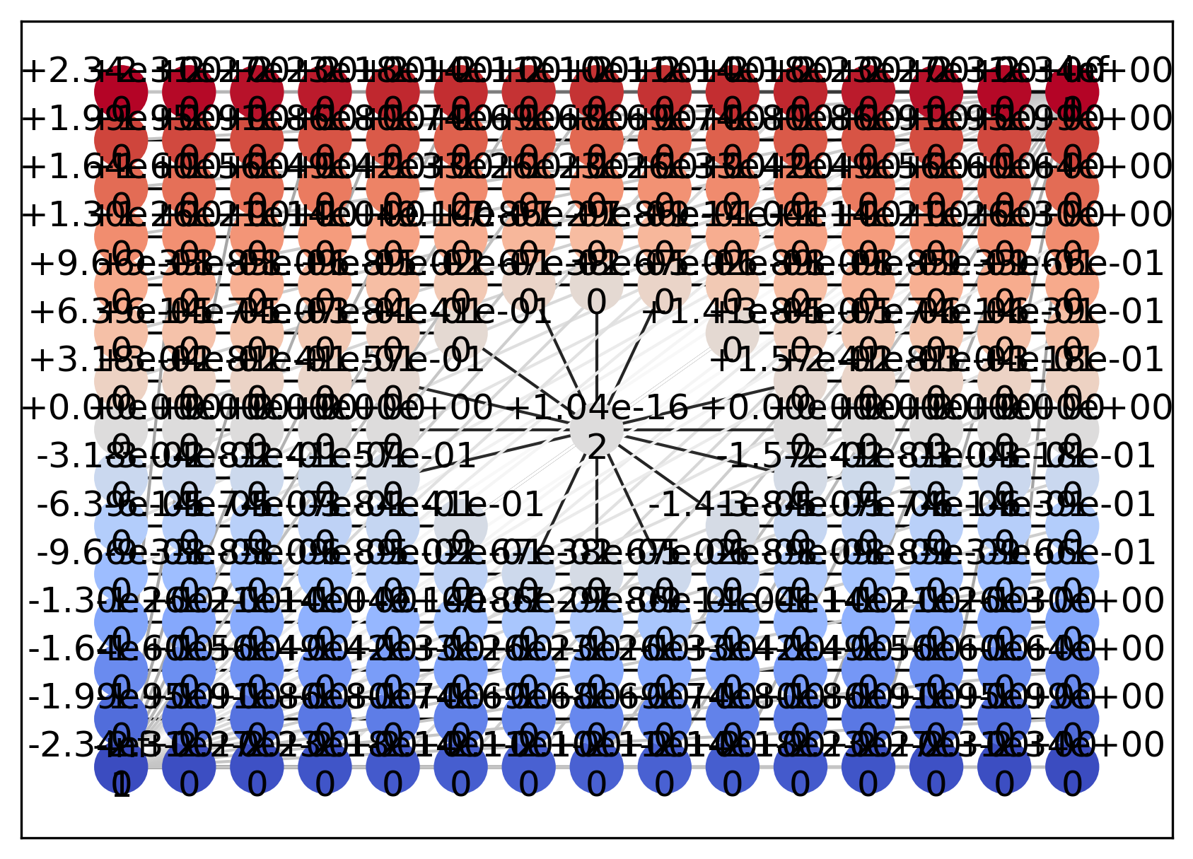
During computation, Psi2tree modifies the adjacency structure of the input data space in order to adjust topological boundary conditions.
As a result, multiple edges can be observed not only around the inner boundary but also around the outer boundary.
Unless you specifically need to inspect such topological structures directly, do not use bitmap=False.
psiclone.visualization.draw_contour()
The draw_contour() function draws contour plots of the input data space.
For more detailed customization of the visualization, use functions such as matplotlib.pyplot.contour() directly.
vis.draw_contour(psi2tree, bitmap=True)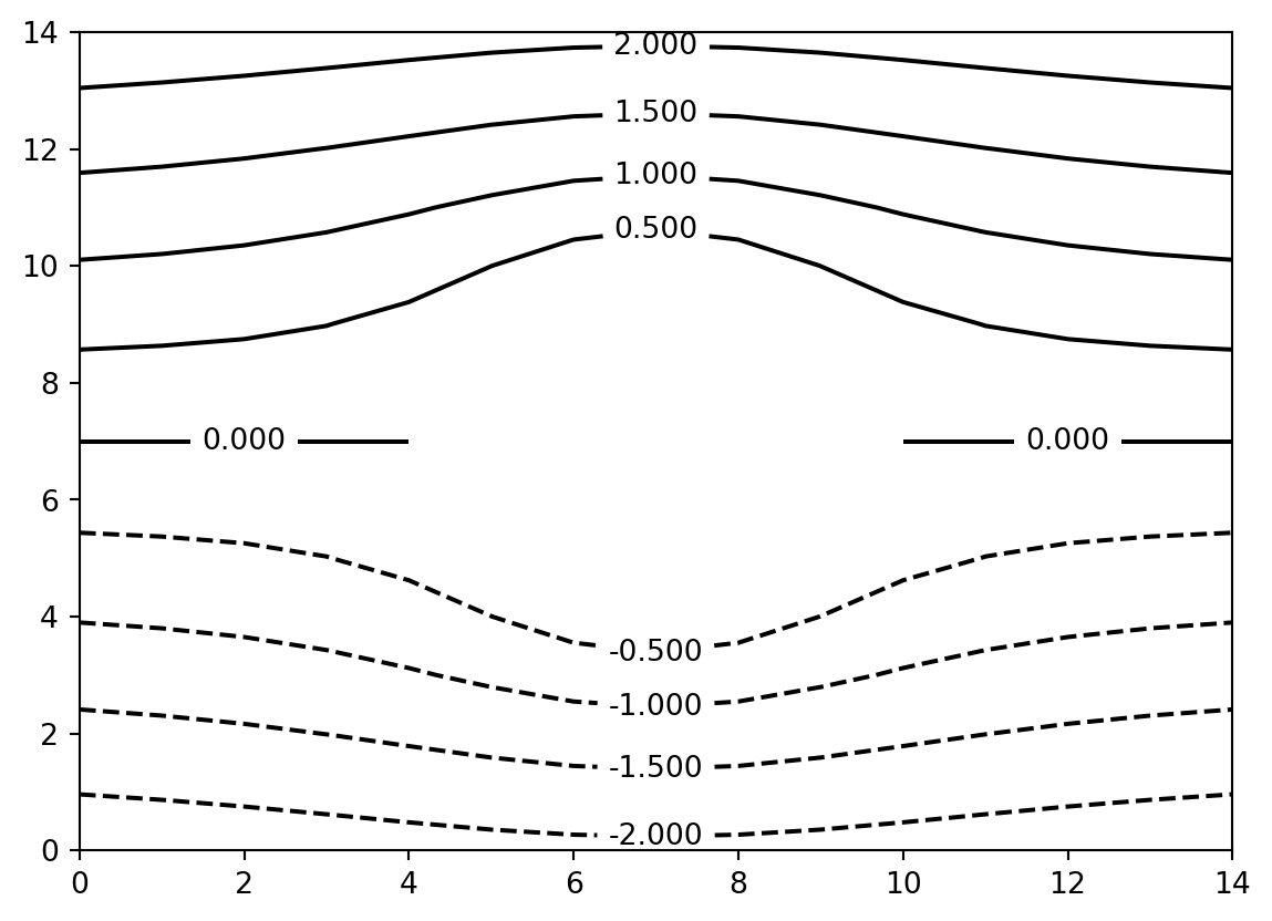
psiclone.visualization.draw_partition()
The draw_partition() function draws the partition diagram obtained from the computation result of Psi2tree.
This corresponds to the equivalence class decomposition induced by the Reeb graph.
vis.draw_partition(psi2tree, bitmap=True)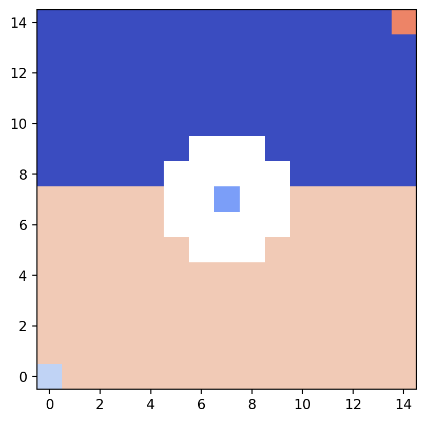
In the partition diagram, different equivalence classes are colored distinctly for easy identification.
Although few in number, pixels corresponding to Reeb graph nodes are also assigned different colors.
psiclone.visualization.draw_graph_markers()
The draw_graph_markers() function draws the Reeb graph in the coordinate system of the input data space.
In the example below, note that the drawing coordinate range is explicitly specified to match the input data space coordinates, instead of using the default integer coordinates.
vis.draw_bitmap(
    geom,
    # Specify extent so that it matches the coordinates of the input data space
    extent=[x0, x1, y0, y1],
)
vis.draw_graph_markers(psi2tree, lw=3, edge_color="y-", node_color="g*")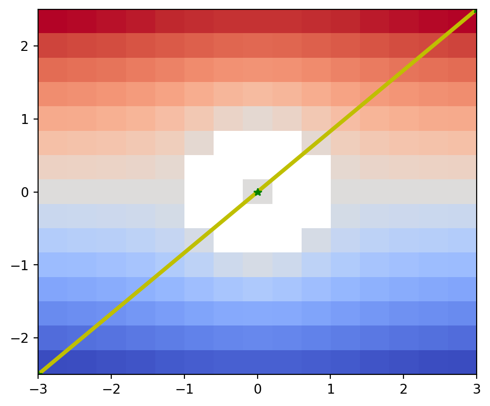
psiclone.visualization.draw_COT_labels()
The draw_COT_labels() function draws the corresponding COT labels near each edge of the Reeb graph.
vis.draw_partition(
    psi2tree,
    bitmap=True,
    # Specify extent so that it matches the coordinates of the input data space
    extent=[numpy.amin(x), numpy.amax(x), numpy.amin(y), numpy.amax(y)],
)
vis.draw_graph_markers(psi2tree, lw=1)
vis.draw_COT_labels(psi2tree)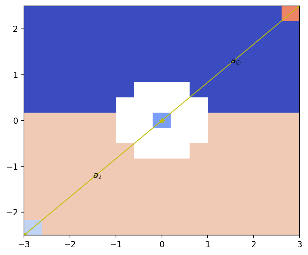
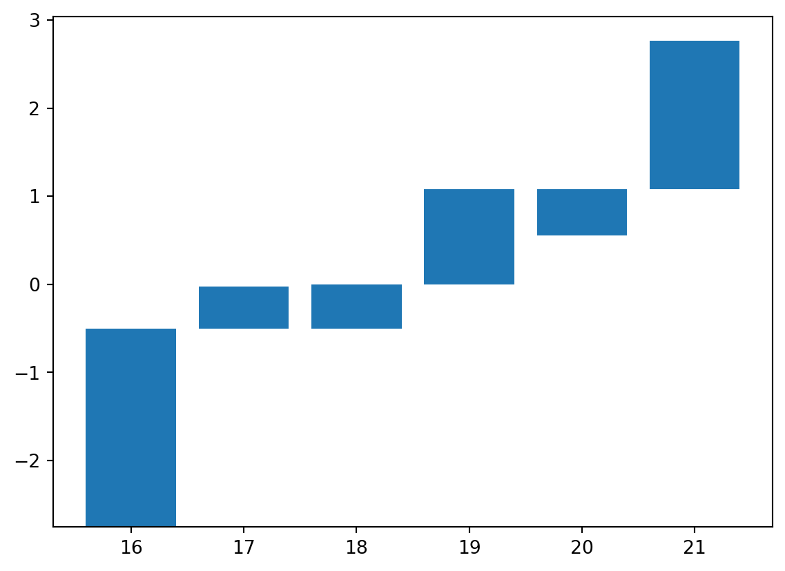
psiclone.visualization.draw_barcode()
The draw_barcode() function draws barcode diagrams for persistent homology and the Reeb graph computed from the input data space.
vis.draw_barcode(psi2tree)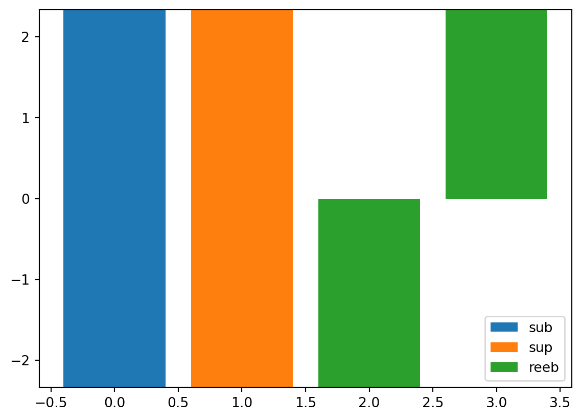
From left to right:
- Barcode diagram of sublevel-set filtration persistent homology
- Barcode diagram of superlevel-set filtration persistent homology
- Barcode diagram of the Reeb graph
A barcode diagram represents each edge of a height-annotated graph as a bar spanning the corresponding height interval.
Advanced Visualization Methods
We now examine how to use functions for more advanced visualization.
First, we modify the input data to make it slightly more complex.
x0, x1, y0, y1 = -3.0, 3.0, -2.5, 2.5
# A real number specifies the step width; an integer multiplied by an imaginary unit specifies the number of divisions
dx, dy = 129j, 129j
x, y = numpy.mgrid[x0:x1:dx, y0:y1:dy]
z = x + y * 1j
flow_domain = numpy.abs(z) >= 1.0
obstacle_domain = ~flow_domain

z = numpy.ma.masked_array(z, obstacle_domain)
W = z + 1.0 / z
perturbation = numpy.zeros_like(x)
perturbation += 0.2 * y
perturbation += 0.3 * numpy.ma.log(numpy.abs(z - (2.0 + 2.0j)))
perturbation -= 0.3 * numpy.ma.log(numpy.abs(z - (2.0 - 1.5j)))
data = numpy.imag(W) + flow_domain * perturbation

table = numpy.ma.masked_array([x, y, data]).reshape((3, -1)).T
geom = convert_array_to_geometry(table, obstacles=[(0, 0)], int_grid=False)
next(node for node in geom.nodes if node.geotype == 2).level = 0.0
psi2tree = Psi2tree(geom, threshold=0.1)
psi2tree.compute()

vis.draw_bitmap(geom)
plt.title(psi2tree.get_tree().convert(to_str))
plt.show()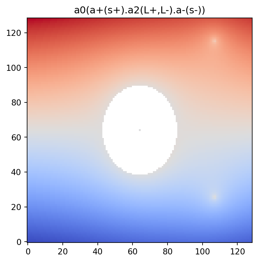
psiclone.visualization.get_partition_data()
The get_partition_data() function retrieves information about the equivalence class decomposition induced by the Reeb graph.
This corresponds to the data used by draw_partition() and consists of a triple: partition, vmin, and vmax.
The partition is a list of classification values derived from the height (level) values of the input data space.
partition, vmin, vmax = vis.get_partition_data(psi2tree)

# Transpose flow_domain (ij-indexing) before drawing
plt.imshow(flow_domain.T, origin="lower", cmap="gray")
vis.draw_bitmap(geom, node_color=partition, vmin=vmin, vmax=vmax)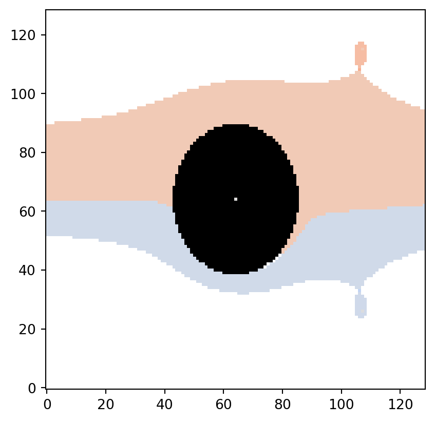
Here, since Psi2tree performed computation for a uniform flow, virtual points with level values of \(\pm\infty\) (points at infinity) are added to the input data space geom.
As a result, some equivalence classes take values of \(\pm\infty\).
Topologically, the leftmost downstream region corresponds to the \(+\infty\) equivalence class, while the rightmost corresponds to the \(-\infty\) equivalence class.
The values vmin and vmax are not derived from partition, but instead represent the minimum and maximum among the bounded level values of the original input data.
If the minimum or maximum is topologically close to the outer boundary, it may be classified as \(\pm\infty\), and thus vmin or vmax may not actually appear in partition.
When drawing the partition diagram with a color range consistent with the original data, it is advisable to make appropriate use of vmin and vmax.
vmin, numpy.amin(data), vmax, numpy.amax(data)(np.float64(-2.763353687123051),
np.float64(-2.7529496539518234),
np.float64(2.763353687123051),
np.float64(2.763353687123051))Additionally, due to noise removal, the partition may contain regions that are “unclassified.”
These are represented as None within partition.
# Count the number of None entries
len([i for i, x in enumerate(partition) if x is None])5If discrete=True is specified, the equivalence class decomposition is represented using newly assigned integer values instead of the original level values of the input data.
In this case, the values \(\pm\infty\) are not included.
Accordingly, partition becomes a list of optional int values.
plt.imshow(flow_domain.T, origin="lower", cmap="gray")
partition, vmin, vmax = vis.get_partition_data(psi2tree, discrete=True)
vis.draw_bitmap(geom, node_color=partition, vmin=vmin, vmax=vmax)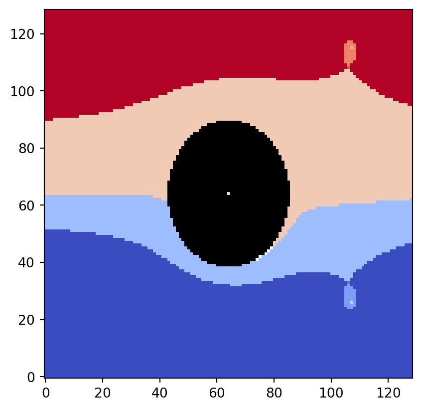
psiclone.visualization.get_COT_constructions()
The get_COT_constructions() function retrieves the recursive construction of the COT representation along with the corresponding Reeb graph equivalence class information.
It returns a dictionary-like object where COT node objects serve as keys and the associated equivalence class information is stored as values.
constructions = vis.get_COT_constructions(psi2tree)
for cot_node, partition in constructions.items():
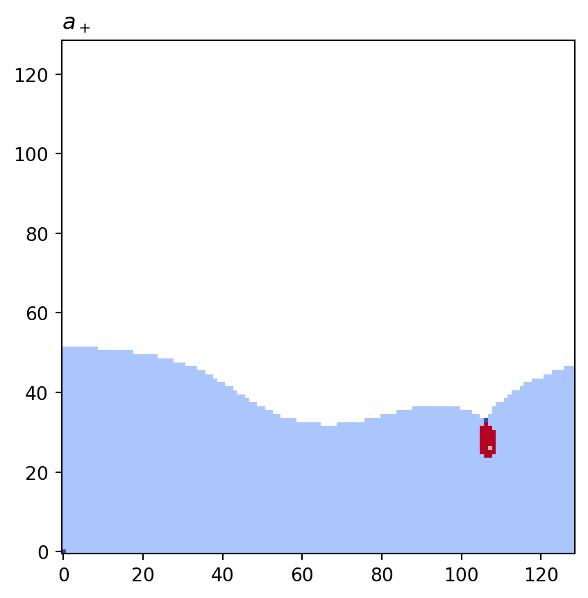
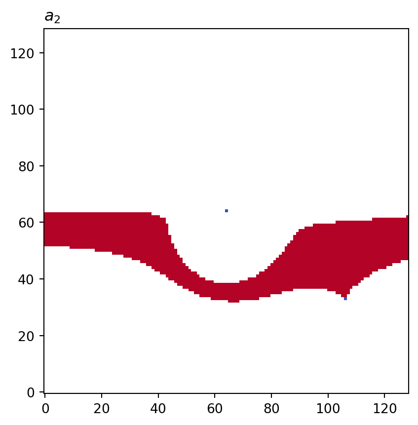
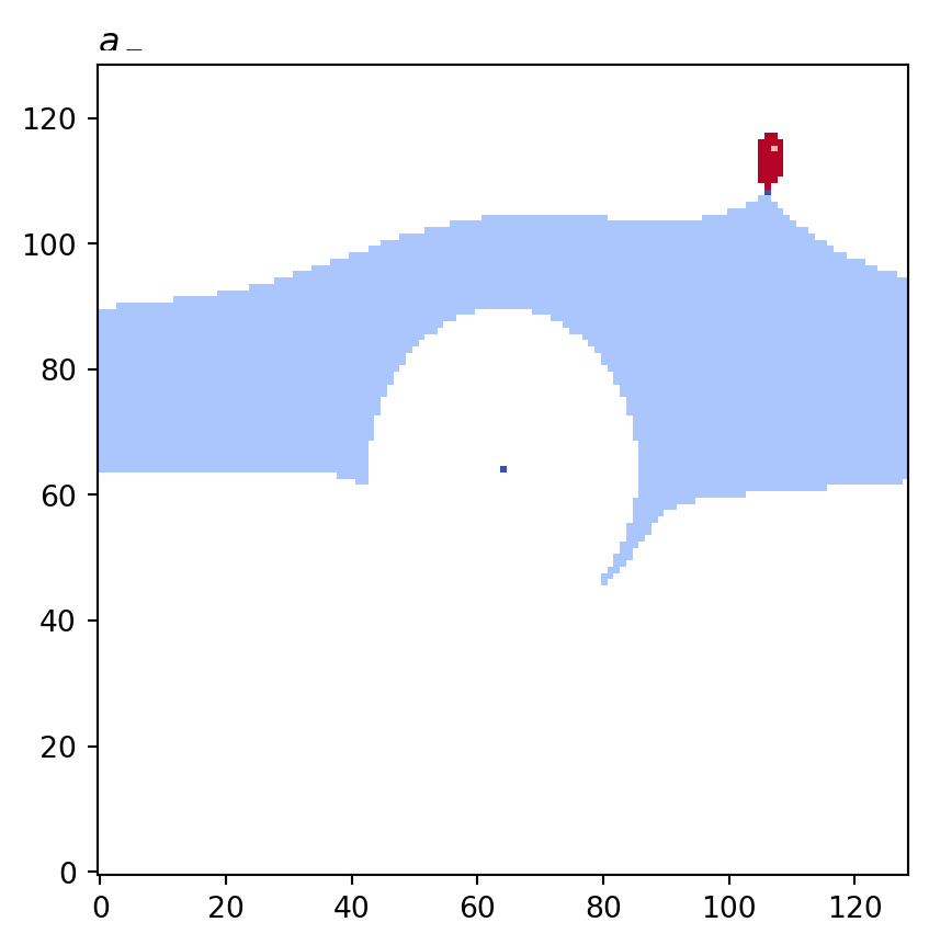
print(f"{cot_node.label()}: key={cot_node}\tvalue={numpy.array(partition)}")a0: key=<psiclone.cot.TreeA0 object at 0x7f3a35ac04d0> value=[3 3 3 ... 4 2 0]
a+: key=<psiclone.cot.TreeA object at 0x7f3a35a52930> value=[1 1 1 ... None 0 None]
s+: key=<psiclone.cot.Genus object at 0x7f3a35acca70> value=[None None None ... None None None]
a2: key=<psiclone.cot.TreeA2 object at 0x7f3a35736810> value=[None None None ... 0 None None]
a-: key=<psiclone.cot.TreeA object at 0x7f3a35ac37a0> value=[None None None ... 0 None None]
s-: key=<psiclone.cot.Genus object at 0x7f3a35b42e70> value=[None None None ... None None None]Each equivalence class is represented as a list of optional float values with the same size and ordering as the node array of the input data space.
cot_node = next(iter(constructions.keys()))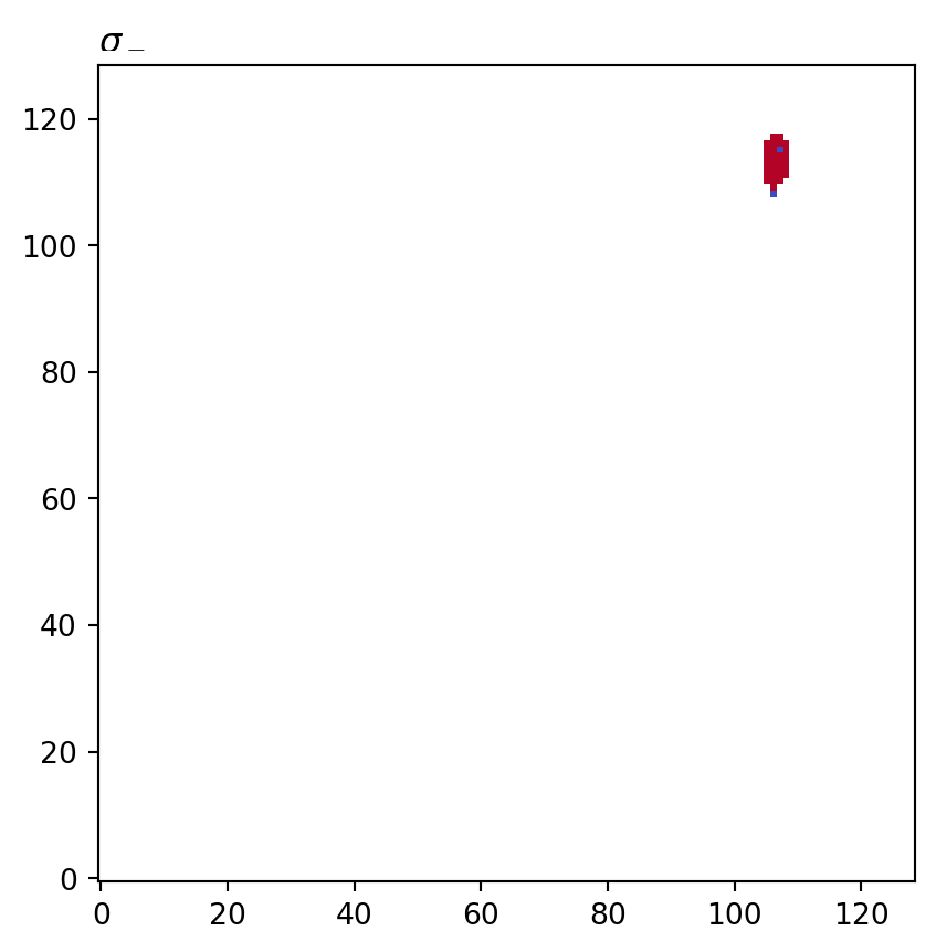
len(constructions[cot_node]) == len(geom.nodes)TrueThese lists can be passed to the node_color option of draw_bitmap or draw_geometry.
for cot_node, partition in constructions.items():
    tex = cot_node.label(tex=True)
    vis.draw_bitmap(geom, title=f"${tex}$", node_color=partition)
    plt.show()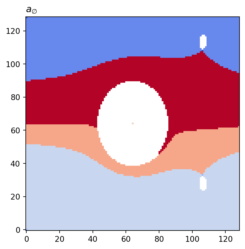
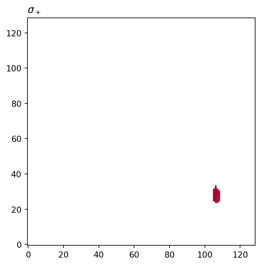
psiclone.visualization.get_graph_markers_data()
The get_graph_markers_data() function retrieves the information needed to draw the Reeb graph in the coordinates of the input data space.
This corresponds to the data used by draw_graph_markers() and consists of a pair: lines and points.
lines, points = vis.get_graph_markers_data(psi2tree)

vis.draw_partition(psi2tree, bitmap=True, extent=[x0, x1, y0, y1])
for line in lines:
    plt.plot(line[0], line[1], "black", lw=1)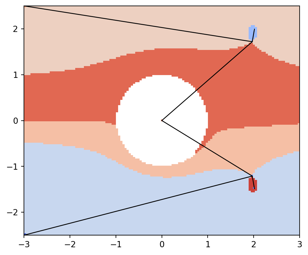
vis.draw_partition(psi2tree, bitmap=True, extent=[x0, x1, y0, y1])
plt.scatter(points[:, 0], points[:, 1], s=150, c="black", marker="*")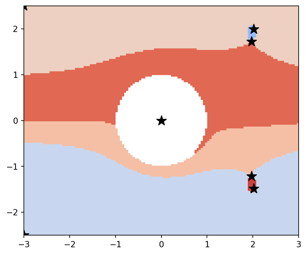
psiclone.visualization.get_barcode_data()
The get_barcode_data() function retrieves barcode information.
This corresponds to the data used by draw_barcode() and returns a dictionary-like object with keys 'sub', 'sup', and 'reeb'.
These represent barcode data for sublevel persistent homology, superlevel persistent homology, and the Reeb graph, respectively.
Each barcode is represented as a triple of arrays: x, y0, and y1.
Here, x is the index of each bar, y0 is the lower bound of the bar, and y1 is the upper bound.
vis.get_barcode_data(psi2tree){'sub': (array([0, 1]),
array([-2.75294965, 0.55322506]),
array([2.76335369, 1.08143079])),
'sup': (array([ 2, 3, 4, 5, 6, 7, 8, 9, 10, 11, 12, 13, 14, 15]),
array([-0.02617826, 0.00358474, 0.01381636, 0.02492754, 0.03030266,
0.03121934, 0.05834316, 0.06569003, 0.06629733, 0.07192172,
0.07369314, 0.07440814, 0.07892039, 2.76335369]),
array([-0.50588341, -2.75294965, -2.75294965, -2.75294965, -2.75294965,
-2.75294965, 0.02752536, 0.06562705, 0.02152453, 0.03687794,
0.05984956, 0.04302202, 0.05388596, -2.75294965])),
'reeb': (array([16, 17, 18, 19, 20, 21]),
array([-2.75294965, -0.50588341, -0.50588341, 0. , 0.55322506,
1.08143079]),
array([-0.50588341, -0.02617826, 0. , 1.08143079, 1.08143079,
2.76335369]))}x, y_bottom, y_top = vis.get_barcode_data(psi2tree)["reeb"]
plt.bar(x, y_top - y_bottom, bottom=y_bottom)