Handling 2D Mesh (Unstructured Grid) Data

Although psiclone does not directly support loading mesh (unstructured grid) data, it is still possible to perform computations on arbitrary unstructured meshes by directly constructing a Geometry object. Specifically, one can add nodes and edges to a Geometry object and then use it as input to Psi2tree. Below we describe the complete workflow.

import numpy

from psiclone.data import Geometry, GrayscaleImage
from psiclone.visualization import draw_geometry

First, let us convert a GrayscaleImage into a Geometry object and examine what kind of data structure this object holds.

img = GrayscaleImage(numpy.arange(12).reshape((3, 4)))
geom = img.to_geometry()
geom.nodes

[Point(id=np.int64(0), level=np.int64(0), x=np.int64(0), y=np.int64(0), geotype=np.int64(1), order=np.float64(-2.498091544796509)),
 Point(id=np.int64(1), level=np.int64(1), x=np.int64(1), y=np.int64(0), geotype=np.int64(1), order=np.float64(-2.1587989303424644)),
 Point(id=np.int64(2), level=np.int64(2), x=np.int64(2), y=np.int64(0), geotype=np.int64(1), order=np.float64(-1.5707963267948966)),
 Point(id=np.int64(3), level=np.int64(3), x=np.int64(3), y=np.int64(0), geotype=np.int64(1), order=np.float64(-0.982793723247329)),
 Point(id=np.int64(4), level=np.int64(4), x=np.int64(0), y=np.int64(1), geotype=np.int64(1), order=np.float64(-2.896613990462929)),
 Point(id=np.int64(5), level=np.int64(5), x=np.int64(1), y=np.int64(1), geotype=np.int64(0), order=np.float64(nan)),
 Point(id=np.int64(6), level=np.int64(6), x=np.int64(2), y=np.int64(1), geotype=np.int64(0), order=np.float64(nan)),
 Point(id=np.int64(7), level=np.int64(7), x=np.int64(3), y=np.int64(1), geotype=np.int64(1), order=np.float64(-0.4636476090008061)),
 Point(id=np.int64(8), level=np.int64(8), x=np.int64(0), y=np.int64(2), geotype=np.int64(1), order=np.float64(2.896613990462929)),
 Point(id=np.int64(9), level=np.int64(9), x=np.int64(1), y=np.int64(2), geotype=np.int64(1), order=np.float64(2.677945044588987)),
 Point(id=np.int64(10), level=np.int64(10), x=np.int64(2), y=np.int64(2), geotype=np.int64(1), order=np.float64(1.5707963267948966)),
 Point(id=np.int64(11), level=np.int64(11), x=np.int64(3), y=np.int64(2), geotype=np.int64(1), order=np.float64(0.4636476090008061))]

draw_geometry(geom)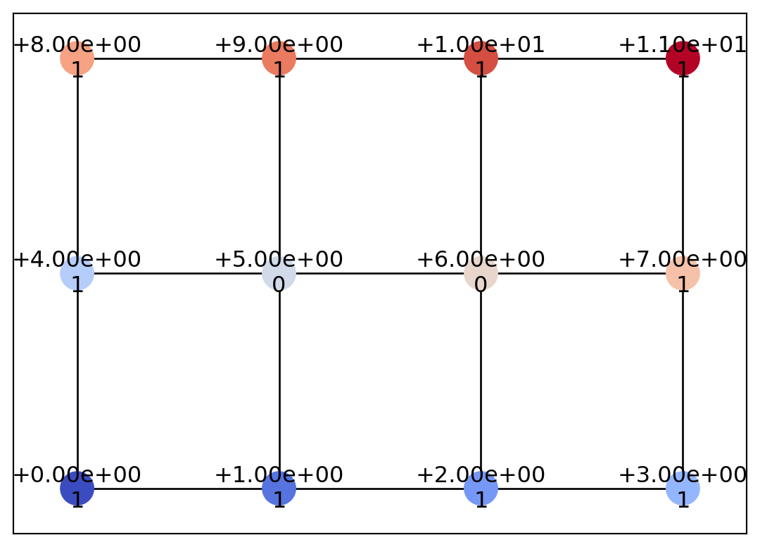

As shown above, a GrayscaleImage object (or the Geometry object obtained by converting the GrayscaleImage) is composed of a grid graph based on the von Neumann neighborhood (four-directional connectivity). Here, let us add “diagonal” edges to this graph.

for i in range(2):
    for j in range(3):
        idx = 4 * i + j
        geom.add_edge(geom.nodes[idx], geom.nodes[idx + 5])

draw_geometry(geom, edge_color="k")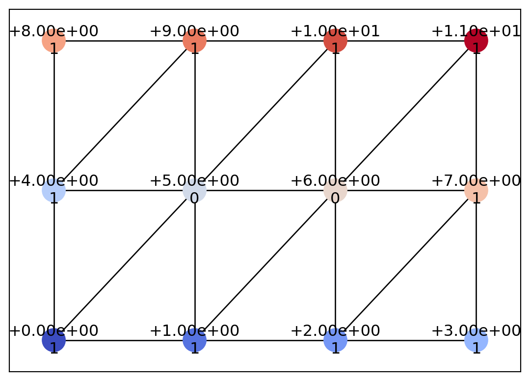

In this way, we have constructed a triangular mesh. The COT representation algorithm in psiclone is based on scalar values defined on a graph and on the adjacency structure of that graph. Therefore, even if scalar data are defined on the same spatial coordinates, the computation results may vary based on the graph’s adjacency structure.

In addition, since Geometry is simply graph-structured data, it does not have to consist of triangles only, as shown in the following example.

from psiclone.data import Geotype

ex_node = geom.add_node(id=12, x=4.5, y=1, level=-1, geotype=Geotype.EXTERIOR)
geom.add_edge(ex_node, geom.nodes[3])
geom.add_edge(ex_node, geom.nodes[11])
draw_geometry(geom, edge_color="k")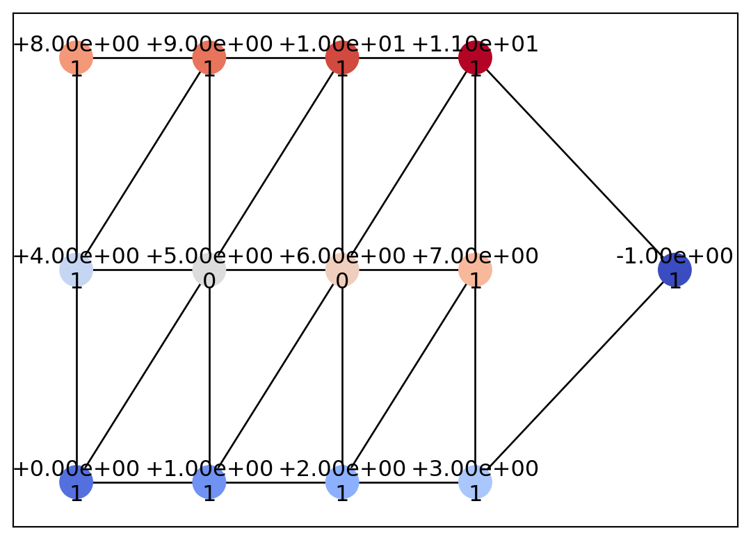

Let us now look at a more practical example of computing a COT representation from mesh data. Here, we define data on a Delaunay triangulation using scipy.spatial.Delaunay. For details on Delaunay(), please refer to the SciPy documentation.

import matplotlib.pyplot as plt
from scipy.spatial import Delaunay

# Generate Delaunay triangulation from random points
num_points = 20
points = numpy.random.rand(num_points, 2)
tri = Delaunay(points)

plt.triplot(points[:, 0], points[:, 1], tri.simplices)
plt.plot(points[:, 0], points[:, 1], "o")
plt.show()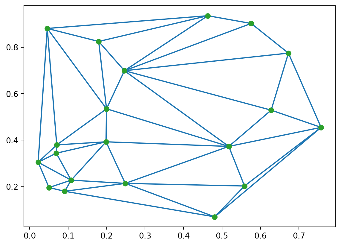

Using the randomly generated point set points, we generated a Delaunay triangulation with the scipy.spatial.Delaunay() function. The result is stored in the object tri. The triangle (simplex) data are stored in tri.simplices, where each simplex is a triplet of node indices. Based on this information, we add nodes and edges to an empty Geometry object.

Each node in Geometry requires some additional information. The geotype attribute should be set to Geotype.INTERIOR for interior nodes of the input domain, and to Geotype.EXTERIOR for boundary (external) nodes. Depending on the boundary conditions of the data, the order attribute may also be required. Furthermore, if the input domain is not simply connected but multiply connected, additional values must be assigned to the geotype attribute (see Analyzing bounded flows using psiclone.util.mcdomain for details). In this example, we set only the geotype attribute based on tri.convex_hull.

mesh = Geometry()


def f(x, y):
    return x**2 + numpy.cos(8 * y)


boundary_indices = set(numpy.unique(tri.convex_hull))

for i, (x, y) in enumerate(tri.points):
    geotype = Geotype.EXTERIOR if i in boundary_indices else Geotype.INTERIOR
    mesh.add_node(id=i, x=x, y=y, level=f(x, y), geotype=geotype)

has_edge = numpy.zeros((num_points, num_points), dtype="bool")
for simplex in tri.simplices:
    for a, b in zip(simplex, numpy.roll(simplex, 1), strict=False):
        if has_edge[a, b]:
            continue
        mesh.add_edge(mesh.nodes[a], mesh.nodes[b])
        has_edge[a, b] = has_edge[b, a] = True

draw_geometry(mesh, edge_color="k")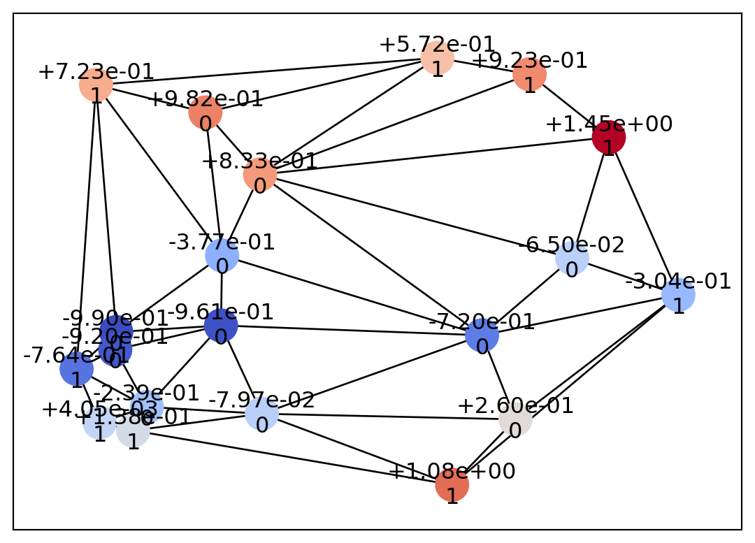

This completes the setup of the input domain data. The remaining step is to process this input data using Psi2tree.

from psiclone.cot import to_str
from psiclone.psi2tree import Psi2tree

psi2tree = Psi2tree(geom, threshold=0.0)
psi2tree.compute()
psi2tree.get_tree().convert(to_str)

'a0(L~)'

The data has now been successfully converted into a COT representation.

Other Formats