The `psiclone.util` Module

psiclone provides the psiclone.util module for handling input spatial data with complex geometries. The main functions are as follows:

psiclone.util.convert.convert_array_to_geometry() – Converts tabular grid data with missing values into a multiply connected domain.
psiclone.util.mcdomain.mcdomain_to_geometry() – Converts grid data with missing values into a multiply connected domain.

Both functions are designed under the assumption that the input space is a multiply connected domain. However, if you are working with a simply connected rectangular domain without missing values, consider using GrayscaleImage instead of this module.

	`GrayscaleImage()`	`convert_array_to_geometry()`	`mcdomain_to_geometry()`
Input domain	Simply connected rectangular domain	Multiply connected rectangular domain	Multiply connected domain
Grid type	Uniform grid (integer coordinates)	Non-uniform grid (non-integer coordinates allowed)	Uniform grid (integer coordinates)
Suitable flow	Uniform flow / bounded flow	Uniform flow / bounded flow	Bounded flow
Input data format	2D array (image)	Tabular data with $x, y, ψ (x, y)$	2D array
Internal obstacles (boundaries)	Not supported	User specifies representative obstacle points	Obstacles detected automatically
Missing / mask support	Not supported	Supported	Supported
Boundary value of $ψ$	User specified	Automatically computed via `numpy.average`	Computation method specified via option

Each method has its own advantages and disadvantages, and an appropriate choice must be made depending on the situation. In particular, boundary handling is crucial in TFDA, and incorrect boundary settings may lead to unexpected analytical results. The functions in the util module are intended only for simplified analyses; verifying boundary conditions for each specific case is essential. If you need to handle input data with more complex geometric structures, please also refer to Handling Mesh-Structured Data.

import matplotlib.pyplot as plt
import numpy

Analyzing Uniform Flow Using `psiclone.util.convert`

Using the psiclone.util.convert.convert_array_to_geometry() function, we load input data consisting of multiple (x, y, z) entries under a setting with a single obstacle placed at the center, and convert it into the COT representation of a uniform flow.

import psiclone.visualization as vis
from psiclone.psi2tree import Psi2tree

Here, the input space is taken to be an unbounded domain with a circular exclusion. However, while it is theoretically unbounded, we treat it as truncated to a suitable rectangular region to make it bounded.

y, x = numpy.mgrid[-3:3:101j, -3:3:101j]
z = x + y * 1j
flow_domain = numpy.abs(z) >= 1.0
obstacle_domain = ~flow_domain

plt.imshow(flow_domain, cmap="gray", origin="lower")

We created a mesh grid and defined the complex variable $z = x + y \sqrt{- 1}$ using the imaginary unit 1j. We consider the flow domain ${z : | z | \geq 1}$ , representing a flow region with a circular obstacle at the center.

To represent data over this domain, it is convenient to use numpy.ma.masked_array. This is a special array type that allows missing regions to be specified using a mask. Except for masked regions, it behaves like a standard numpy.ndarray. Using the complex variable $z$ and a masked_array, we define the stream function as follows.

z = numpy.ma.masked_array(z, obstacle_domain)
W = z + 1.0 / z
data = numpy.imag(W)
plt.imshow(data, cmap="coolwarm", origin="lower")
plt.contour(data, colors="k")

We have now created test data representing uniform flow around a circular obstacle. Next, we convert this into a Geometry object.

table = numpy.ma.masked_array([x, y, data]).reshape((3, -1)).T
table.shape

(10201, 3)

We use the utility function psiclone.util.convert.convert_array_to_geometry() to construct a Geometry object under a uniform flow setting with an obstacle. For this purpose, we first prepare masked tabular data of size $N \times 3$ consisting of $x, y, ψ (x, y)$ . (Instead of a masked array, you may also use nan to represent missing regions, or simply omit entries corresponding to missing regions.)

This function has several optional arguments. Here, we specify only one representative coordinate for the obstacle via the obstacles argument. It is sufficient to provide a single representative point for each obstacle. In this example, we specify the origin.

from psiclone.util.convert import convert_array_to_geometry

geom = convert_array_to_geometry(table, obstacles=[(0, 0)])
geom, len(geom.nodes), len(geom.edges)

(<psiclone.data.geometry.Geometry at 0x7f086c3b35c0>, 9325, 18476)

The data for the input space has now been prepared. Let us check whether the constructed geom corresponds to the same data as shown above.

vis.draw_geometry(geom, bitmap=True)

Observe carefully that the representative point specified at the center of the obstacle is drawn. This pixel is assigned the average value of the boundary data along the internal boundary. Let us inspect the attribute values of the obstacle node. Obstacle nodes are assigned a geotype value of 2 or higher (Geotype.OTHERS).

from psiclone.data import Geotype

obstacle_node = next(node for node in geom.nodes if node.geotype >= Geotype.OTHERS)
obstacle_node

Point(id=9324, level=np.float64(-1.1825031694575236e-16), x=0, y=0, geotype=2, order=nan)

You can confirm that the level value of the obstacle node is close to $0$ . It is not exactly $0$ due to discretization effects. Since it is set as the average of the stream function values at grid points along the internal boundary, small numerical errors arise.

With convert_array_to_geometry, boundary conditions (stream function values at the boundary) cannot be specified in advance. If the input data is obtained from numerical computation and the exact boundary data is known beforehand, you should explicitly set the level values of the added boundary nodes. If this value deviates significantly from the ideal boundary condition, it may not be possible to compute an appropriate COT representation near the boundary. However, if the data resolution is sufficiently high, such small numerical errors can usually be ignored in practice.

obstacle_node.level = 0.0  # Reset because the exact boundary value is known (optional)

The input space data geom is now fully prepared.
Let us compute the COT representation using Psi2tree.

psi2tree = Psi2tree(geom, threshold=0.0)
psi2tree.compute()

After the computation is complete, obtain the result using the get_tree method.
The tree structure returned by get_tree can then be converted into a human-readable format using the convert method.

from psiclone.cot import to_str

psi2tree.get_tree().convert(to_str)

'a0(a2(L+,L-))'

The symbol a2 represents the flow that collides with the central obstacle.
This confirms that we have successfully represented uniform flow data with a single obstacle at the center.

Analyzing Bounded Flow Using `psiclone.util.mcdomain`

Next, we examine an example of constructing a multiply connected domain using the psiclone.util.mcdomain.mcdomain_to_geometry() function.
mcdomain stands for “multiply connected domain.”
Following the same procedure as before, we now use an annular region as the input space.

y, x = numpy.mgrid[-3:3:101j, -3:3:101j]
z = x + y * 1j
flow_domain = numpy.logical_and(numpy.abs(z) >= 1.0, numpy.abs(z) < 3.0)
obstacle_domain = ~flow_domain

plt.imshow(flow_domain, cmap="gray", origin="lower")

On this annular domain, we define a test scalar function.
Here, we artificially impose the outer boundary condition $z = 0$ .

z = x**2 + x + 1.5 * y**2
z *= x**2 + y**2 - 9  # 外側境界条件 z = 0 を強制
data = numpy.ma.masked_array(z, obstacle_domain, fill_value=numpy.nan)
plt.imshow(data, cmap="coolwarm", origin="lower")
plt.contour(data, colors="k")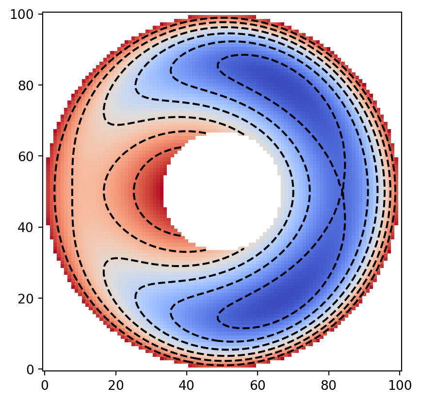

We specify the outer boundary condition using the boundary_condition option so that the outer boundary value becomes zero.
You may directly specify 0, or since the scalar values increase outward, specifying 'max' yields the same effect.

Due to discretization, unintended fine noise often appears around boundaries in the streamline topology.
The 'max' and 'min' options are convenient for effectively suppressing such discretization effects.

On the other hand, when capturing characteristic structures such as streamline topology near the inner boundary, 'average' or 'mean' may be more suitable than 'max' or 'min'.
It is important to choose appropriate boundary conditions depending on the situation.

from psiclone.util.mcdomain import mcdomain_to_geometry

yi, xi = numpy.indices(data.shape)
geom = mcdomain_to_geometry(
    xi.ravel(),
    yi.ravel(),
    data.ravel(),
    boundary_condition=[
        (Geotype.EXTERIOR, "max"),  # Outer boundary condition; you may also specify 0 directly
        (Geotype.OTHERS, "average"),  # Inner boundary condition
    ],
)

/opt/build/repo/.venv/lib/python3.12/site-packages/psiclone/util/mcdomain.py:67: UserWarning:

Warning: converting a masked element to nan.

vis.draw_geometry(geom, bitmap=True)
plt.colorbar()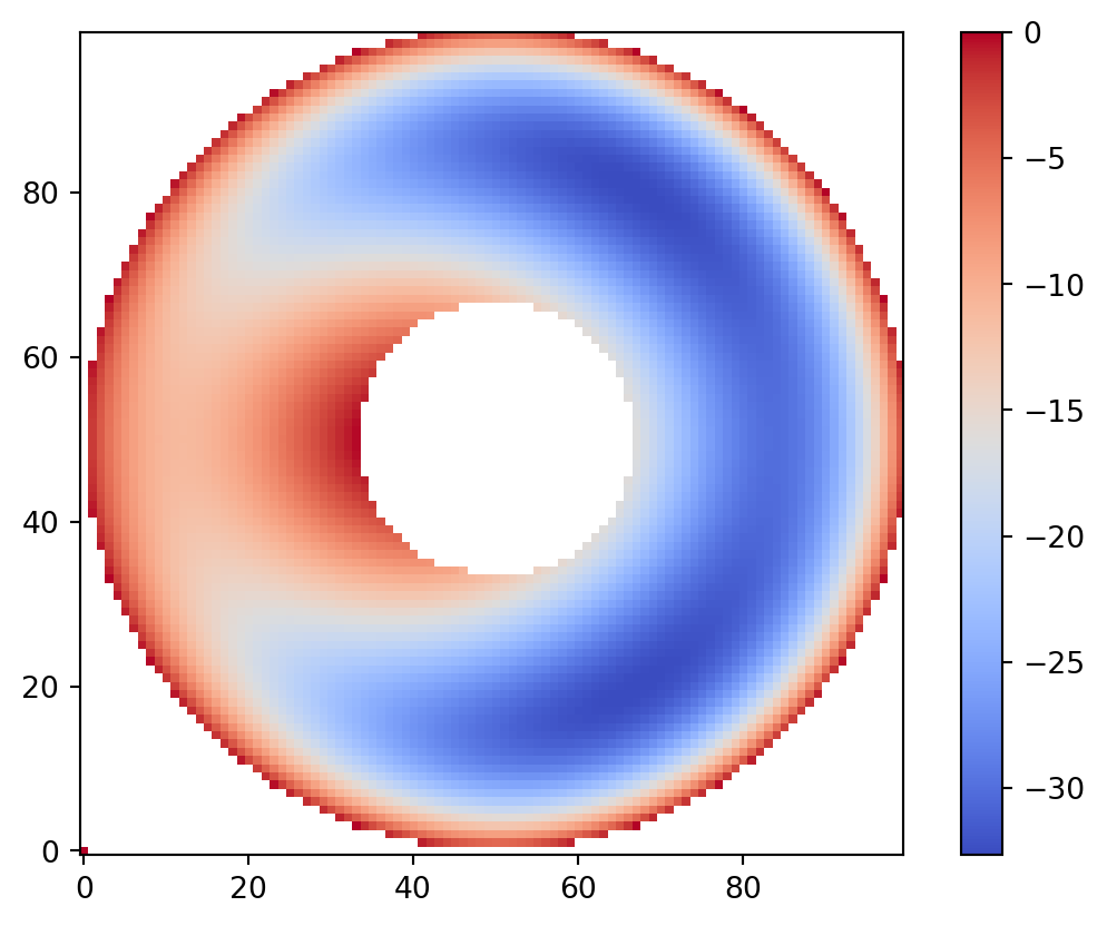

Now we perform the computation and output the partition diagram and the COT representation.

from psiclone.cot import to_short_tex

psi2tree = Psi2tree(geom, threshold=1.0)
psi2tree.compute()
title = psi2tree.get_tree().convert(to_short_tex)

vis.draw_partition(psi2tree, bitmap=True, title=f"${title}$")
vis.draw_graph_markers(psi2tree)
vis.draw_COT_labels(psi2tree)

Analyzing Uniform Flow Using psiclone.util.convert

Analyzing Bounded Flow Using psiclone.util.mcdomain

Analyzing Uniform Flow Using `psiclone.util.convert`

Analyzing Bounded Flow Using `psiclone.util.mcdomain`